Important: Please read Lab Guidelines before you continue.
This lab consists of 3 exercises. You are required to submit 2 exercises. If you submit 3 exercises, the best 2 out of 3 exercises will be used to determine your attempt mark.
The main objective of this lab is on the use of two-dimensional arrays to solve problems.
The maximum number of submissions for each exercise is 10.
If you have any questions on the task statements, you may post your queries on the relevant IVLE discussion forum. However, do not post your programs (partial or complete) on the forum before the deadline!
Important notes applicable to all exercises here:
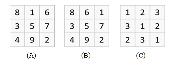
A semi-magic square is an n x n matrix of integers if 1) all the row sums and column sums are the same, and 2) it includes all integers from 1 to n2.
For example, let say n is 3, as shown below, matrix A is a 3 x 3 semi-magic square since all the row sums and column sums are the same (= 15), and it includes all integers between 1 to 9.
In contrast, matrix B is not a semi-magic square because its middle column sums to 20 while its right column sums to 10.
Lastly, matrix C is not a semi-magic square either because it includes integers 1 to 3 but not 4 to 9.
Write a program square.c to perform the following:
Your program should have a function called scanSquare() for reading in the inputs, and a function called isSemiMagic() for checking the square. You are to determine the parameters.
Sample runs using interactive input (user's input shown in blue; output shown in bold purple). Note that the first two lines (in green below) are commands issued to compile and run your program on UNIX.
Sample run #1:
$ gcc -Wall square.c -o square
$ square
Enter size of square: 3
Enter values in the square:
8 1 6
3 5 7
4 9 2
It is a semi-magic square.
Sample run #2:
$ gcc -Wall square.c -o square
$ square
Enter size of square: 3
Enter values in the square:
8 6 1
3 5 7
4 9 2
It is not a semi-magic square.
The time here is an estimate of how much time we expect you to spend on this exercise. If you need to spend way more time than this, it is an indication that some help might be needed.
(This exercise is adapted from AY2013/14 PE2 Exercise 2.)
Given a 12×12 board which contains integer values in the range [1, 9], and a particular search digit in the same range, write a program sequence.c to find the longest sequence of this search digit in the board.
The sequence can be horizontal (left to right →), vertical (top to bottom ↓), or diagonal (north-west to south-east ↘). Your program will report the length of this longest sequence, and where (which row and column) the sequence starts. When there are more than 1 sequence with the same longest length, you should report the one that starts closest to row 0 column 0, according to row-major order (where all elements in row r are closer to row 0 column 0 than elements in row r+1).
Your program should contain at least 2 functions:
The sample runs below show the same board, with different search digits. However, your program will be tested on different boards.
Sample run using interactive input (user's input shown in blue; output shown in bold purple). Note that the first two lines (in green below) are commands issued to compile and run your program on UNIX.
Sample run #1:
The solution sequence is shown in red below for easy indentification.
$ gcc -Wall sequence.c -o sequence
$ sequence
3 6 7 7 3 4 7 9 2 7 7 7
6 1 1 1 1 4 7 2 8 7 2 3
6 6 4 8 2 2 7 7 6 2 3 8
8 1 3 8 3 6 6 2 1 7 4 3
6 2 3 8 8 8 7 8 9 7 1 8
7 9 1 6 8 6 8 2 9 3 2 8
1 2 6 3 1 9 6 6 7 8 1 6
2 6 7 9 8 9 7 6 4 8 1 6
6 4 8 3 9 4 1 3 9 2 4 4
1 6 6 3 1 1 6 8 4 8 1 1
4 8 1 7 8 9 7 6 7 4 6 3
2 2 2 9 4 3 3 1 3 4 4 2
1
Length of longest sequence = 4
Start at (1,1)
Sample run #2:
The two sequences with length 3 are shown in red below. The solution is the sequence that starts at (0,6) instead of the one that starts at (0,9), since (0,6) is nearer to (0,0) than (0,9).
3 6 7 7 3 4 7 9 2 7 7 7
6 1 1 1 1 4 7 2 8 7 2 3
6 6 4 8 2 2 7 7 6 2 3 8
8 1 3 8 3 6 6 2 1 7 4 3
6 2 3 8 8 8 7 8 9 7 1 8
7 9 1 6 8 6 8 2 9 3 2 8
1 2 6 3 1 9 6 6 7 8 1 6
2 6 7 9 8 9 7 6 4 8 1 6
6 4 8 3 9 4 1 3 9 2 4 4
1 6 6 3 1 1 6 8 4 8 1 1
4 8 1 7 8 9 7 6 7 4 6 3
2 2 2 9 4 3 3 1 3 4 4 2
7
Length of longest sequence = 3
Start at (0,6)
Sample run #3:
3 6 7 7 3 4 7 9 2 7 7 7
6 1 1 1 1 4 7 2 8 7 2 3
6 6 4 8 2 2 7 7 6 2 3 8
8 1 3 8 3 6 6 2 1 7 4 3
6 2 3 8 8 8 7 8 9 7 1 8
7 9 1 6 8 6 8 2 9 3 2 8
1 2 6 3 1 9 6 6 7 8 1 6
2 6 7 9 8 9 7 6 4 8 1 6
6 4 8 3 9 4 1 3 9 2 4 4
1 6 6 3 1 1 6 8 4 8 1 1
4 8 1 7 8 9 7 6 7 4 6 3
2 2 2 9 4 3 3 1 3 4 4 2
6
Length of longest sequence = 3
Start at (5,5)
Sample run #4:
3 6 7 7 3 4 7 9 2 7 7 7
6 1 1 1 1 4 7 2 8 7 2 3
6 6 4 8 2 2 7 7 6 2 3 8
8 1 3 8 3 6 6 2 1 7 4 3
6 2 3 8 8 8 7 8 9 7 1 8
7 9 1 6 8 6 8 2 9 3 2 8
1 2 6 3 1 9 6 6 7 8 1 6
2 6 7 9 8 9 7 6 4 8 1 6
6 4 8 3 9 4 1 3 9 2 4 4
1 6 6 3 1 1 6 8 4 8 1 1
4 8 1 7 8 9 7 6 7 4 6 3
2 2 2 9 4 3 3 1 3 4 4 2
3
Length of longest sequence = 2
Start at (2,10)
Sample run #5:
3 6 7 7 3 4 7 9 2 7 7 7
6 1 1 1 1 4 7 2 8 7 2 3
6 6 4 8 2 2 7 7 6 2 3 8
8 1 3 8 3 6 6 2 1 7 4 3
6 2 3 8 8 8 7 8 9 7 1 8
7 9 1 6 8 6 8 2 9 3 2 8
1 2 6 3 1 9 6 6 7 8 1 6
2 6 7 9 8 9 7 6 4 8 1 6
6 4 8 3 9 4 1 3 9 2 4 4
1 6 6 3 1 1 6 8 4 8 1 1
4 8 1 7 8 9 7 6 7 4 6 3
2 2 2 9 4 3 3 1 3 4 4 2
5
No such sequence.
The time here is an estimate of how much time we expect you to spend on this exercise. If you need to spend way more time than this, it is an indication that some help might be needed.
The Game of Life – a simulation 'game', not an interactive game that involves players – is invented by the British mathematician John H. Conway in 1970. In a rectangular grid in which each cell is either empty (a dead cell) or occupied by an organism (a live cell), we see how the population evolves through a series of generations, according to these rules:
Consider the following example in Figure 2:
![]()
Figure 2. Game of Life
Cells A and C will die of loneliness in the next generation as each of them has only one neighbour, while cell B will survive. Cells D and E will be born in the next generation as each of them has three neighbours in the current generation.
You are to write a program life.c to implement the Game of Life on a rectangular grid of 20 rows by 20 columns. Your program should read the data for the initial generation, which we shall call generation 0. The data are characters, where 'O' (captial O) denotes a live cell, and '-' (hyphen) denotes a dead cell. You may assume that there is at least 1 live cell in generation 0.
Your program is to generate up to the fifth generation and display the fifth generation. If the community dies down (that is, no live cell exists) before it reaches the fifth generation, you should stop and display that generation. If the community is identical to its previous generation, you should also stop and display that generation.
For example, in sample run #1 below, generation 3 is identical to generation 2, hence the program stops at generation 3 and displays it.
Tip: Using sentinels
Because the cells have different number of neighbours (8, 5 or 3) depending on
their locations, your code has to consider these different cases. To simplify your
code, the idea of sentinels, a common technique in programming, can be
employed here. Instead of declaring your array as a 20 rows by 20 columns, you
declare it as a 22 × 22 array so that you have an additional "boundary"
of cells surrounding the 20 × 20 area, which is the actual population.
The boundary can be filled with dead cells. Your code will examine only
the 20 × 20 area, in which case all the cells in this area have exactly
8 neighbours each. This idea of using sentinels makes the code neater, at the
expense of a little extra space used. The skeleton program given assumes the
use of sentinels.
Sample run using interactive input (user's input shown in blue; output shown in bold purple). Note that the first two lines (in green below) are commands issued to compile and run your program on UNIX.
Sample run #1:
$ gcc -Wall life.c -o life
$ life
--------------------
--------------------
--------------------
--------------------
--------------------
--------------------
--------------------
--------------------
--------------------
--------OOOO--------
--------------------
--------------------
--------------------
--------------------
--------------------
--------------------
--------------------
--------------------
--------------------
--------------------
Generation 3:
--------------------
--------------------
--------------------
--------------------
--------------------
--------------------
--------------------
--------------------
---------OO---------
--------O--O--------
---------OO---------
--------------------
--------------------
--------------------
--------------------
--------------------
--------------------
--------------------
--------------------
--------------------
Sample run #2:
--------------------
--------------------
--------------------
--------------------
--------------------
--------------------
--------------------
--------------------
--------------------
-------OOOOO--------
--------------------
--------------------
--------------------
--------------------
--------------------
--------------------
--------------------
--------------------
--------------------
--------------------
Generation 5:
--------------------
--------------------
--------------------
--------------------
--------------------
--------------------
---------O----------
--------OOO---------
-------O-O-O--------
------OOO-OOO-------
-------O-O-O--------
--------OOO---------
---------O----------
--------------------
--------------------
--------------------
--------------------
--------------------
--------------------
--------------------
Figure 3 below shows the 15 test cases. For better visual effect, the dead cells are shown as blanks below. There are even names given to some of the input patterns!
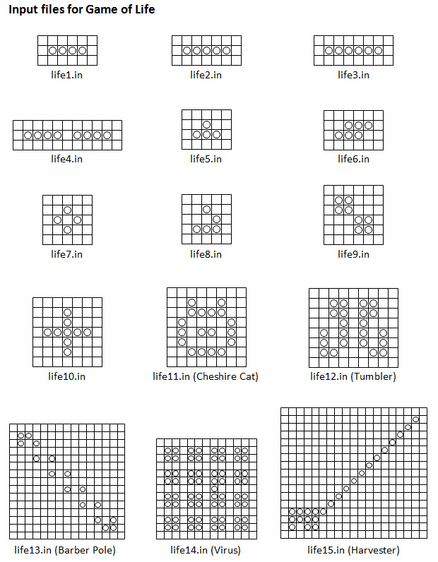
Figure 3. Test cases for Game of Life
The time here is an estimate of how much time we expect you to spend on this exercise. If you need to spend way more time than this, it is an indication that some help might be needed.
A compiled demo program is provided here: life_demo
This program has been compiled in sunfire and hence it can only run in sunfire. It uses curses, a terminal control library for UNIX-like systems consisting of functions that manage an application's screen display. If you are interested, google it.
You may download this program and test it on the input files provided. For example: life_demo < life15.in
Some of the input files above are interesting. There are patterns that oscillate infinitely after a few generations, such as life2.in, life5.in, life6.in, life9.in, and life13.in.
There are patterns where the live cells all die off after some generations, such as life3.in and life10.in.
The deadline for submitting all programs is 25 October 2017, Wednesday, 5pm. Late submission will NOT be accepted.