Experiments of Probabilistic Model Checking
Multi-agent Behaviors in Dispersion Game
This webpage is used to give more
details of the experiments in Probabilistic
Model Checking Multi-agent Behaviors in Dispersion Game. All the examples
are available here.
We use model checker PAT to
fulfill these experiments on a PC with 2 Intel Xeon CPUs at 2.13GHz and 32GB
RAM, and in the following are two strategies of dispersion game we use in our
paper, which is a typical example of multi-agent learning problem.
・
Experiments compared
with PRISM model checker
Basic
Simple Strategy[1]
BSS is a novel
strategy for agents to make decisions in repeated dispersion game proposed by Alpern. This strategy is only
suitable for the case when the number of agents n is
equal to the number of actions. In each round, the agent simultaneously choose
their actions in a probabilistic manner based on the outcome of previous round.
For this case, we are focusing on two
properties: convergence and convergence rate.
Convergence: this is to check the probability that the BSS strategy will stabilize on an MDO state, which is represent in LTL as System |= <>[] MDO. The results are listed in the following table.
A printable
version of BSS(Agents=Actions=4) model as an example
is available here.
|
System |
Prob of
Converge |
Time (s) |
States |
|
Agents=Actions=3 |
1 |
0.045 |
698 |
|
Agents=Actions=4 |
1 |
0.787 |
8412 |
|
Agents=Actions=5 |
1 |
12.026 |
99168 |
|
Agents=Actions=6 |
1 |
945.853 |
1211808 |
|
Agents=Actions=7 |
1 |
67421 |
14925310 |
Table 1: Converge
probability for BSS system.
From Table 1, we could conclude that for BSS strategy, it will always
encounter a convergence state which is an MDO state. The state space and
verification times are growing rapidly when the number of actions increases.
1.
Convergence rate: this is used to check
how fast the converge could occur in terms of the
number of rounds the strategy executes. We slightly change the BSS model by
adding a round counter to record which round the system is in. The property is
represented as System
reaches MDO’, and MDO’ is defined as get into the MDO state within
a specific number of rounds. The results are shown in figure 1.
A printable
version of BSS(Agents=Actions=4, round counter added)
model as an example is available here.
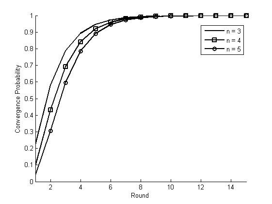
Figure 1: Convergence probability
within different rounds in BSS with different number of agents n
From Figure 1, we could conclude that for BSS strategy, after 14 rounds,
the system will get into the MDO state with probability 1. The
smaller of the number of actions, the faster.
Extended Simple Strategy[2]
ESS is an extension of
BSS in the way that the number of agents could be more than the number of
actions, which is studied in[2].
For this case, we are also focusing
on two properties: convergence and convergence rate.
1. Convergence: this is to check the probability that the ESS strategy will stabilize on an MDO state, which is represent in LTL as System |= <>[] MDO. The results are listed in Table 3.
A printable
version of ESS(Agents=4, Actions=2) model as an
example is available here.
|
System |
Prob of
Converge |
Time (s) |
States |
|
Agents=3, Actions=2 |
0 |
0.222 |
204 |
|
Agents=3, Actions=3 |
1 |
0.239 |
698 |
|
Agents=4, Actions=2 |
1 |
0.229 |
316 |
|
Agents=4, Actions=3 |
0 |
0.459 |
2337 |
|
Agents=4, Actions=4 |
1 |
1.119 |
7176 |
|
Agents=5, Actions=2 |
0 |
0.246 |
580 |
|
Agents=5, Actions=3 |
0 |
1.312 |
4880 |
|
Agents=5, Actions=4 |
0 |
8.957 |
29076 |
|
Agents=6, Actions=2 |
1 |
0.238 |
800 |
|
Agents=6, Actions=3 |
1 |
1.302 |
7196 |
|
Agents=6, Actions=4 |
0 |
103.87 |
69558 |
|
Agents=7, Actions=2 |
0 |
0.289 |
1262 |
|
Agents=7, Actions=3 |
0 |
6.238 |
16108 |
|
Agents=7, Actions=4 |
0 |
816.54 |
145972 |
|
Agents=8, Actions=2 |
1 |
0.454 |
1628 |
|
Agents=8, Actions=3 |
0 |
30.189 |
26763 |
|
Agents=8, Actions=4 |
1 |
196.42 |
206216 |
|
Agents=9, Actions=2 |
0 |
0.567 |
2342 |
|
Agents=9, Actions=3 |
1 |
20.806 |
35228 |
|
Agents=9, Actions=4 |
0 |
8679.7 |
516322 |
|
Agents=10, Actions=2 |
1 |
1.083 |
2892 |
|
Agents=10, Actions=3 |
0 |
120.53 |
64390 |
|
Agents=10, Actions=4 |
0 |
44111 |
925340 |
Table 2: Converge
probability for ESS system.
From Table 3, we could conclude that for ESS strategy, in some cases the
system cannot get into a convergence state. This is decided by the relation
between the number of agents and the number of actions. This phenomena
inspires us to explore another interesting property in ESS: what is the
probability that after getting into a MDO state, the system will exit from it
in the following round?
The property is represented as System |=! MDO U (MDO && X(m) !MDO), which means system will entrance an MDO state and then in the next round, it exits from it. The results are displayed by the following figure.
|
System |
Prob of
Exit from MDO |
Time (s) |
States |
|
Agents=3, Actions=2 |
0.063 |
0.019 |
99 |
|
Agents=3, Actions=3 |
0 |
0.023 |
347 |
|
Agents=4, Actions=2 |
0 |
0.008 |
156 |
|
Agents=4, Actions=3 |
0.073 |
0.204 |
1162 |
|
Agents=4, Actions=4 |
0 |
0.136 |
3586 |
|
Agents=5, Actions=2 |
0.070 |
0.037 |
286 |
|
Agents=5, Actions=3 |
0.125 |
0.472 |
2429 |
|
Agents=5, Actions=4 |
0.122 |
1.575 |
14516 |
|
Agents=6, Actions=2 |
0 |
0.019 |
398 |
|
Agents=6, Actions=3 |
0 |
0.217 |
3596 |
|
Agents=6, Actions=4 |
0.152 |
11.439 |
34740 |
|
Agents=7, Actions=2 |
0.074 |
0.083 |
626 |
|
Agents=7, Actions=3 |
0.091 |
1.246 |
8037 |
|
Agents=7, Actions=4 |
0.158 |
43.975 |
72938 |
|
Agents=8, Actions=2 |
0 |
0.037 |
812 |
|
Agents=8, Actions=3 |
0.137 |
5.357 |
13360 |
|
Agents=8, Actions=4 |
0 |
2.854 |
103106 |
|
Agents=9, Actions=2 |
0.069 |
0.326 |
1165 |
|
Agents=9, Actions=3 |
0 |
0.482 |
17612 |
|
Agents=9, Actions=4 |
0.137 |
130.4 |
258059 |
|
Agents=10, Actions=2 |
0 |
0.086 |
1444 |
|
Agents=10, Actions=3 |
0.092 |
14.658 |
32163 |
|
Agents=10, Actions=4 |
0.157 |
402.98 |
462530 |
Table 3:
Probability for ESS system to deviate from MDO state.
From table 4, it is desired to see that for those cases whose
convergence probability is 0, they have an exiting
probability from the MDO state. Theoretically speaking, no matter how small the
probability is, in the long run it will eventually get into a non-MDO state,
since infinite loop on a non-1 probability transition is not allowed. However
in practice, since the probability is quite small, we could assume the ESS
system could stabilize on an MDO state.
2. Convergence
rate: this is used to check how fast the converge
could occur in terms of the number of rounds the strategy executes. We slightly
change the ESS model by adding a round counter to record which round the system
is in. The property is represented as System
reaches MDO’, and MDO’ is defined as get into the MDO state within
a specific number of rounds. The results are shown in figure 2.
A printable
version of ESS(Agents=4, Actions=2, round counter
added) model as an example is available here.
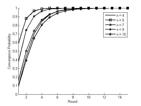
Figure 2: Convergence
Probability for ESS with k = 4
Different
from the results in BSS, when the number of agents n increases, the convergence
probability until each round begins to increase first and gradually decreases.
Experiments compared with PRISM model checker
PRISM is widely used in probabilistic model
checking; meanwhile, there are several works in game theory using PRISM model
checker, which could be found here. The reasons for us to choose PAT in
this work are as follows.
1.
PAT
supports a more complex modeling language. It has some constructs which
guarantee a more compact and convenient approach to build the model. We have
built basic examples of BSS in both PAT and PRISM, and compared with PAT’s
model, PRISM’s state based language leads to a much larger structure, which
will take users more effort to build a suitable model. This could be found in
the following PRISM example.
A printable
version of BSS(Agents= Actions=4) model of
PRISM as an example is available here.
What is more, as the number of actions increases, the
lines of code(LOC) of PAT’s model will increase
linearly meanwhile LOC of PRISM’s model will increase exponentially, so we only
build the above example in PRISM.
2. Another important factor in model checking is its
efficiency. To compare the efficiency between PRISM and PAT, we use the above
PRISM model to check the probability that BSS(N=4)
will get into convergence state, which is the same property we check in PAT System
|= <>[] MDO.
PRISM takes more than 2 seconds to get the correct
answer, while PAT just takes 0.787 seconds, which could be found in table 1.
Actually for LTL checking, PAT has some optimized algorithms, so that this kind
of better efficiency is expected. More cases could be found in [3].
|
Agents= Actions=4 |
Pr(System|=<>[]MDO) |
Time(s) |
States |
|
PRISM |
1 |
2.296 |
8412 |
|
PAT |
1 |
0.787 |
8552 |
According to the above
reasons, we choose PAT as our model checker in this work in order to get a more
efficient verification result.
References
1. S. Alpern. Spacial dispersion as a dynamic
coordination problem. Technical
report, The London School of Economics, 2001
2.
Y.
S. T. Grenager, R. Powers. Dispersion games:
general definitions and some specific learning results. In Eighteenth National Conference on
Artificial intelligence (2002),
pages 398--403. 2002
3.
J. Sun, S. Song,
and Y. Liu.
Model checking hierarchical probabilistic systems. In Proceeding of the 12th International
Conference on Formal Engineering Methods, ICFEM 2010, pages 388-403. 2010