Constraint propagation on the continuous domain involves heavy use of interval arithmetic. The constraints are usually expressed in the form of intervals, which are propagated through the system using the equations that define the system.

However, two problems have plagued computations that use interval arithmetic. First is the observation that interval arithmetic does not take into account the appearance of identical variables. Suppose we have a variable x, which has the interval [0, 1] (where 0 denotes its lower limit and 1 is the upper limit). Performing interval arithmetic on the equation x – x will give the interval [-1, 1], when the actual interval should be [0, 0]. This is known as the dependency problem and is especially problematic when there are a lot of such equations (such as the Michaelis Menton formulation that is common in the modeling of biological pathways).

The second problem lies with the representation of the constraints and the pessimistic propagation of errors. In the case of a multi-variate system of equations, the most common representation of allowable intervals is in the form of an n-dimensional box. This box does not tightly encapsulate the allowable region and the errors that are propagated will explode such that the interval does not contract. This is known as the wrapping problem. Later on in this short report, we shall see the problems that are generated by such a representation and suggest ways to circumvent it.

As a start, with [1] as a reference, we shall see, step by step, the boxes (constraints on the parameters and variables) that are propagated throughout the pathway during parameter estimation.

Model 1 – Linear Chain

The simplest example for consideration is that of a linear chain. Suppose we have the pathway structure shown below (as a Hybrid Functional Petri Net model). Grey color places indicate known experimental data at discrete time points. 

Figure 1 – Simple linear chain

The system of equations that defines this simple pathway (and the nominal parameters, i.e. parameter values which we will be trying to estimate using just the experimental data) is as shown below.

 Suppose the nominal values of the parameters and the initial conditions of the places are as below.

Table 1 – Experimental data for x₂ 

Table 2 – Experimental data for x₁

By rearranging the variables, the equations can be written in the following forms (Caps are used to denote the interval extensions of their corresponding variables/parameters) 

We shall assume that the original ranges for k₁, k₂ and k₃ are [0.001, 1.0] and that in cases whereby x₁ and its derivative is unknown, their interval will be [0, 5] and [0, 3] respectively. Considering the values for x₁ and x₂ for time = 6, with the first iteration of constraint propagation, we get the intervals: 

The slight reduction in interval comes for the parameters k₁ and k₂. Even after a considerable number of iterations, the resulting interval is still not significantly better.

Via an exhaustive search of the parameters k₁, k₂ and k₃ within the interval [0.001, 1.0], we can see that the actual region is very small, due to the way we encode the intervals of each ‘combination’ of parameters (i.e. n-dimensional box for n parameters), the included error region (region which we know that no solutions exist) is inherently large.

Figure 2 – The actual allowable region (blue) versus the region (region) that can be encapsulated using simply boxes to denote the regions

In this case, we can see that for k₁, k₂ and k₃, the actual allowable region is a small strip of rectangular box, rotated in a certain angle – which brings us to the first question should interval analysis be considered as a viable means of reducing the parameter search space. What should be the representation of a region (other than an n-dimensional box)? 

In a related problem, in the simulation of systems of ODE using interval analysis, one of the most common ways to alleviate this problem is to use a technique known as QR-factorization. However, this is used together with an alternate representation of the ODEs, i.e. Interval Taylor Models (ITS) [2].

Model 2 – Shared Input Place

As an added analysis, we shall see what the parameter space looks like for the configuration where there is a shared input place and a shared outgoing place.  

Consider the pathway configuration below.

Figure 3 – Shared input place

Its corresponding system of equations is then shown below.

Suppose again that the nominal values of the parameters and the initial conditions of the places are as follows

Table 3 – Experimental data for x₁

Table 4 – Experimental data for x₂

Table 5 – Experimental data for x₅

Again, we try out an exhaustive search for the parameters to see which parameters will produce an interval that encompasses the data for time t = 6. The box that covers the solution is:

[0.2, 0.3] (k₁) × [0.04, 0.5] (k₂) × [0.12, 0.74] (k₃) × [0, 0.995] (k₄) × [0.095, 0.995] (k₅)

Considering just the last three variables k3, k4 and k5, again, we can see that the box is relative large (almost equivalent to the original interval that we started out with) when in reality, the actual allowable region is just the small box as shown in the figure below.

Figure 4 – The actual allowable region (blue) for the variables k₃, k₄ and k₅

Model 3 – Shared Output Place

The final basic configuration will be one that has a shared outgoing place.

Figure 5 – Shared output place

The system of equations that describes such a system is then shown below

The nominal values for the parameters and initial conditions are, again, as follows

Table 6 – Experimental data for x₁

Table 7 – Experimental data for x₂

Table 8 – Experimental data for x₃

Performing a similar analysis on all the allowable values of the parameters, we are able to obtain the allowable region for the solution for data at time point t = 6. Again, the actual interval if expressed as an n-dimensional box will be:

[0.1, 0.5] (k₁) × [0.02, 0.46] (k₂) × [0.17, 0.99] (k₃) × [0.01, 0.78] (k₄) × [0.01, 0.995] (k₅)

The actual region, however, is depicted in the figure below.

Figure 6 – The actual allowable region (blue) for the variables k₃, k₄ and k₅

Michaelis Menton

In the above three examples, we have seen that for such networks, the allowable region is a rotated box. However, a careful look at the equations reveal that the relationship between the parameters is linear. Hence it might be worthwhile to look at a more common biochemical equation – i.e. Michaelis Menton equation and see how the parameters will vary.

Suppose the network is now of this form.

Figure 7 – A simple pathway depicting Michaelis Menten relation

Table 6 – Experimental data for x₁

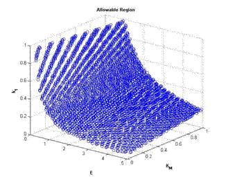
Figure 8 – Allowable regions for variations in the variables k₁, K_M and E.

The allowable region will then be shown in the figure above, i.e. a curved field. This is due to the nonlinear relationship between the parameters k₁ and the concentration of the enzyme E (which in this case we have taken to be a value to be estimated as well).

Parameter Relation

In the above pathway configurations, the allowable regions are due to the relations between the various parameters. Dynamical constraints aside, it is conceivable that there is a range of parameters that will produce similar observations, and these ranges are then related by the equations that define the system, constrained by the observed experimental data. In this section, we shall look at whether or not it is possible to view the constraints not as boxes (or even bounded regions) but from the perspective of the relationship between the parameters.

To do so, we shall just look at some basic structures (non-exhaustive) to get a rough feel of the equations that relate the parameters to one another.

Simple Network

Now we are going to try the full blown example of a simple pathway (using not only a single time point but all the ‘observations’ available) to see if we can, instead of using boxes to represent constraints, find out any relationship between the parameters themselves.

Consider this pathway with a shared enzyme.

Figure 9 – Simple pathway with shared enzyme

Given the pathway, (and using our decompositional approach), there will be 2 overlapping components that will be generated. We do not yet have an objective way of choosing the left component (consisting of x₁, x₂, x₃ and x₄) or the right component (x₁, x₂, x₅ and x₆). Originally, the idea would be to propagate whatever constraints based on the observed values, such that we can ‘randomly’ choose which component to estimate for first. With that, we first give the nominal values for the parameters and generate some ‘experimental data’ (via simulation).

Note that there is conservation of concentration for the variables pairs x₁, x₂ and x₃, x₄ and x₅, x₆. We assume all the pairs sum up to 5.0 nM and initially, all are in the inactive state, i.e. at x₁, x₃ and x₅.

Simulating the system using these parameters will produce the concentration profile shown in the figure below. We shall take discrete time points as our experimental observations.

Figure 10 – Concentration profiles of the variables using the nominal parameters

The discrete time points showing observed values are presented in the table below.

Now we shall form all the equations involving the parameters, keeping in mind that the original range for the parameters are – k in (0, 1.0], K_M in (0, 10.0], V in (0, 10.0].

Since we do not know the values for some of the variables, e.g. x₁, we shall treat them as unknown parameters as well. Putting all the left hand side and right hand sides together, we get (we only need to consider half of the equations as the equations occur in equal and opposite pairs)

By performing a simple substitution, we let the combinations of unknown be represented by y’s, we get. Probably for this case, x₁_dot can be treated as an unknown parameter by itself

The idea of using auxiliary variables is not untested. Kolev L (1999) has tried it out in solving a system of nonlinear equations, converting it instead to a system of linear equations thereafter which can be solved more readily.

Simple Network II

The parhway given above is probably too complicated (for manual computation) due to the presence of additional parameters for the Michaelis-Menton equations. Hence we will consider a simpler version (in terms of equation form as well) where everything is specified in terms of mass action laws.

Similarly, using the following coefficients for nominal values,

We get the following trace for a single experiment

Now we shall form all the equations involving the parameters, keeping in mind that the original range for the parameters are – k in (0, 1.0], and the x’s are in [0, 5.0]. (Red color font denotes variables/parameters whose values are known)

dx₁/dt = –  k₁x₁ + k₂x₂

dx₂/dt =     k₁x₁ –  k₂x₂

dx₃/dt = –  k₃x₂x­₃ + k₄x₄

dx₄/dt =     k₃x₂x­₃ –  k₄x₄

dx₅/dt = –  k₅x₂x­₅ + k₆x₆

dx₆/dt =     k₅x₂x­₅ –  k₆x₆

Re-arranging, we get the following equations

– k₁x₁   + k₂x₂ – dx₁/dt = 0

  k₁x₁   – k₂x₂ – dx₂/dt = 0

– k₃x₂x­₃ + k₄x₄ – dx₃/dt = 0

  k₃x₂x­₃ – k₄x₄ – dx₄/dt = 0

– k₅x₂x­₅ + k₆x₆ – dx₅/dt = 0

  k₅x₂x­₅ – k₆x₆ – dx₆/dt = 0

If taking that x1 and x2 are known (or given a reasonable box), we get

– k₁x₁ + k₂x₂                             – dx₁/dt = 0

  k₁x₁ – k₂x₂                             – dx₂/dt = 0

             – k₃x₂x­₃ + k₄x₄              – dx₃/dt = 0

               k₃x₂x­₃ – k₄x₄               – dx₄/dt = 0

                           – k₅x₂x­₅ + k₆x₆ – dx₅/dt = 0

                             k₅x₂x­₅ – k₆x₆ – dx₆/dt = 0

<Heuristic: Divide constraints into static constraints and dynamical constraints. Static constraints are those that are based on observation and will use interval arithmetic. Dynamical constraints will be like what we are doing now, i.e. plugging in the values and simulating the system and comparing it with experimental trace. Only perform checking via dynamic constraints after checking with the static constraints.>

IDEA IS – Substitute such that I get a system of linear equations based on the parameters (unknown variables are also considered as parameters in this case). Coupled this with a rotation and translation matrix (affine transformation) to allow us to choose parameters in independent parameter space (not the original parameters). Solve for the system of linear equations.

Local Bisection

In this portion, we consider the conventional way of constraint propagation; however we only keep bisection to a local area, i.e. a place and its corresponding transitions. Consider the same pathway configuration.

We compute the possible values (allowable regions) for k₁ and k₂ when considering only the left component, and the allowable regions for the same parameters when considering only the right component. In fact, this is the problem that we have been facing so far, i.e. if we were to estimate for the left component first, we might have chosen values of k₁ and k₂ such that it does not fall into the allowable region for the right component.

Of course when we were to do just constraint propagation without bisection, most likely we would have encountered the ‘wrapping’ problem where, the allowable regions are too pessimistic such that it equals the domain for k₁ and k₂ (such that no information is being extracted from experimental data). What we will do instead, is to consider such constraints locally.

Region Representation

Even within the interval analysis community, there had been a lot of research done to counter the effects of wrapping. Most of them are geometrical solutions, i.e. using ellipsoids, parallelotopes, zonotopes, convex sets, or union of such sets. Based on the simple examples above, we can see that a possible regions representation might possibly be more efficiently expressed as a box, followed by a rotation along the axes. [Update: Those seemingly regular regions are generated via parameters which has linear relationship with one another. For cases whereby the relationship is nonlinear, i.e. power law, Michaelis Menton, it might not necessarily be so]

 However, one thing that needs to be proved is whether or not the allowable region is continuous, i.e. it is not two disjoint sets. 

An Alternative Approach to Choosing Parameters during Parameter Estimation

For most parameter estimation algorithms, they start off with an initial guess of parameters. The constraints that are placed on these initial guesses were simply range checks, i.e. each parameter has an upper and lower bound. However, instead of choosing from such a coarse constraint, it might be better to impose an ordering on the choosing of parameters such that, for each parameter that is chosen, its initial value will contract the range of the other parameters.  

Latest Updates – Use of Interval Newton Contractor to contract the parameter space

Previous work on using interval arithmetic to contract the parameter space has largely failed due to two reasons – Dependency and Wrapping. However, recently we tried a slightly more complicated contracting algorithm – the Interval Newton Contractor, which seems to perform better (but more in-depth analysis is required) in reducing the possible parameter space. It is based on the mean value theorem. Detailed notes can be found here (http://www.ipu.ru/labs/lab7/files/conf05/20-2-2-Walter.pdf).

Reference

[1] Warwick Tucker, Zoltan Kutalik and Vincent Moulton, “Estimating parameters for generalized mass action models using constraint propagation”, submitted to Mathematical Biosciences.

[2] Lubomir V. Kolev, “An Improved Method for Global Solution of Non-Linear Systems”

 For the task of parameter estimation, pathway decomposition is one of the methods to keep complexity of the problem to a manageable level. Decomposition is firstly guided by the need for a component (or sub-graph, which we will use interchangeably) to be executable, with respect to the given experimental data. This being said, it is assumed that the parameters of a component can be initially populated with random values.

 Given a Hybrid Functional Petri Net G = (P, T, A), where P is the set of places, T is the set of transitions and A is the set of arcs connecting the places to transitions and vice versa, a component is a sub-graph G’ = (P’, T’, A’) and it is executable if and only if it is closed under the given conditions:

• Suppose a place p is in the component, if its trajectory is not completely known, then its incoming transitions are also in the component. However if it has outgoing transitions that are connected by Normal arcs, then those outgoing transitions are included in the component.

• Suppose a transition t is in the component, then its incoming places must also be in the component.

 Hence for a biological pathway, there might be several (possibly overlapping) executable components, from which we must determine the order to simulate and estimate such that we maximize the information (in the form of experimental data such as protein concentration) that is given.

 As an additional motivation, in real life situations where there is limited research funding, such a cost function can possibly guide scientists in producing experimental data such that the ‘amount of information’ by those data is maximized, given the (real life) cost constraint.

Cost Function: Scheme 1 (Thiagu)

 In the first scheme, the cost function is guided by the amount of information given to support an unknown parameter in a transition. This can be done simply by scoring, for each transition, the number of surrounding places which have experimental data.

 As a guide, consider the simple example in Figure 1

Figure 1 – Some simple combinations of transitions and places

Consider the simple combination in Figure 1(a). The transition has unknown parameters (denoted by being white in color) and there are no surrounding places with experimental data. Although it is generally true that even places a few hops away might provide some clues on the unknown parameter in that transition, we shall not consider that for the moment. Under such a case, the cost contribution by such a transition should be large, and that it should be proportional to the number of surrounding white places.

 Looking at Figure 1(b) and Figure 1(c), the cost contribution should be less respectively, with the least being Figure 1(c). Of course, each place with experimental data (grey) should be treated differently and a good indication would be the number of experimental points, i.e. the more data points, the less the cost contribution. (Later on these data points might possibly be weighted to reflect the amount of information conveyed, e.g. a series of points at steady state does not contribute any more information as compared to a single point along that state.  But as an initial guide, we shall assume each data point will confer an additional amount of information to the value of the unknown parameter).

 However, the number of data points should not be confused with more ‘grey’ places. For each adjacent place, each data point will reduce the cost, but if there are more grey places, the overall cost should increase. As an example, refer to figures 1(c) and 1(f). Assuming that each grey place has 5 data points, the cost associated to the transition in 1(f) should be more than the cost of that in Figure 1(c).

 In formulating a cost function, we must also take into account the number of unknowns in the transitions. Comparing Figures 1(a) and 1(d), 1(d) should have virtually no cost associated with it as there is nothing to estimate. A convenient measure would be the number of unknowns in the transition, i.e. the cost is directly proportional to the number of unknown parameters. If there are no unknown parameters, this value will then be 0, which will result in 0 cost.

 Hence the cost Cost() associated with a transition t would be

Where

•  is the number of unknown parameters for transition t
•  is the weight assigned to each adjacent place and it is defined to be

 Note that for the weight given to a place with no data points, the 5 is arbitrarily given as we require some sort of penalty that is >1 for such a place. (In most examples that we encounter, it is assumed that the initial conditions are known. This initial condition is counted as one data point. Hence this excessive penalty is given only when there is no knowledge as to what the initial condition of that place will be). For places where we know the trajectory, it can be assumed that there are an infinite number of data points and hence the cost contribution for such a place will be equivalent to 0.

 The cost of a component C is hence the sum of the cost of its individual transitions.

 In the later sections, we will have some sample pathway configurations on which we will try out the various scoring schemes.

Cost Function: Scheme 2 (Lisa)

 An alternative scoring scheme for a component uses the intuition of ‘complexity’ to assess the component. Unlike in the previous scheme where only the transitions are scored, the second scheme takes both places and transitions into consideration. It considers the decomposition problem as producing a set of components for estimation such that the complexity of the components is minimized.

 Although, currently as it stands, ‘complexity’ is yet-to-be defined, but like the previous cost function, it is a property that increases with increased number of unknown parameters within a component. Similarly, it is inversely proportional to the number of data points available. Although seldom encountered, if a place does not have any data points (not even the initial conditions), then an arbitrarily large penalty will have to be assigned to its complexity.

 However, one additional feature that it has (which is not present in the first scheme) is that it takes the connectivity of a place into consideration when computing it. Simply put, for the same number of data points, if they are used to estimate more parameters, the complexity would be higher.

Figure 2 – Complexity of different places

 Referring to Figure 2, assuming that the number of data points for the configuration in 2(a) is the same as that in 2(b), we can say that the ‘complexity’ for estimating the parameters in 2(b) is higher as there are more parameters to be estimated, given the data points.

 Hence for the second scoring scheme, we can define a function Cmplx() which takes in either a  place p or transition t, and is defined as follows:

• , where  is the number of unknown parameters in t.

• , where  is the number of unknown parameters that it is directly connected to (Currently it is set to be the number of arcs to transitions with unknown parameters), However if there are no unknown parameters that uses this place, then its ‘complexity’ will be 1 (In future development, there will be a difference between places which are not connected to any transitions and places that are connected to transitions with known parameters).  is the contribution of the data points (or lack of them) to the complexity of the place, and it is defined to be

 The rationale for having such a form for  is as follows. If there are no data points,  should give a sufficiently small value such that it increases the overall complexity of the component. This value is given by  where . Furthermore, should the number of data points increase,  should increase (to decrease the overall ‘complexity’ contribution) to reflect the intuition that more data points reduces ‘complexity’. However, there should be a limit as to when additional data points do not make any difference to the complexity. This is given by . Its coefficient will determine the number of data points that will cause the total complexity to reduce instead of increase. Hence  will typically be between 1 and 2. (Currently we shall set  to be 1.3 and to be 0.2)

The cost of a component C is hence

 Note that currently this is an incomplete formulation as there should be some other points to consider, such as reconciliation when the components are summed up together. However it does reflect the relationship between the number of data points, the connectivity of the component with the overall ‘complexity’ of the component.

Some Examples

 We try the two scoring schemes on some simple pathway configurations to see what kind of score they produce.

So which scheme better reflects the properties of what a cost function should entail?

David's note:

I would suggest you consider this question. given a single enzyme-catalyzed reaction modeled with Michaelis-Menton equation, how much data (time evolution, steady-state, whatever) do you need to estimate the parameter? the answer should give us a start on defining a notion of cost for estimating the cost of a component.

Original Idea (naive): The idea of having the ratio of 'knowns' vs 'unknowns' as a measure to determine the 'cost' of a component.

Some thoughts and ideas:

• Why not use a transition (parameter) and give it a score according to the number of neighbors known?
• Or alternatively, use a place instead, and assuming that it is known, see how the surrounding parameters can vary, i.e. degrees of freedom
   

• Using an analytic means to predict the outcome of simulation. Motivation: Using numerical integration techniques might be too time consuming, especially for parameter estimation where typically the model will have to be simulated several times.
• Outcome: The simple analytic solution can be worked out, but the more complex one, like a unimolecular conversion-deconversion might pose some problems.

• Work out some standard pathways for use as a benchmark next time
• Three step metabolic pathway
• HIV Protease
• Insulin Signaling Pathway
• Krebs Cycle
• Synthetic pathways

• Dependency Graph
• Since upstream components are possibly restricted by downstream components, are we right to say that there is a dependency of upstream to downstream components?

Notes on Constraint Propagation

Warning: In general, tasks posed in constraint satisfactory problems (CSP) are computationally intractable (NP-HARD) (http://ktiml.mff.cuni.cz/~bartak/constraints/constrsat.html)

Some questions to ask:

• Is there any differences between a dependency graph and a constraint graph? (i.e can we use them interchangeably). If the answer is yes, then there are more operations that we can perform using the dependency graph.
• But the important thing really is to... KEEP THINGS SIMPLE!! Be careful not to complicate issues by adding in too many items. If can do constraints using dependency graph, use it, do not come up with more graphs to mess up the issue.

Concepts of a propagator - function from constraint store (domain) to constraint store (range). It is only allowed to 'contract' , i.e. remove values from constraint store (which is pretty straight forward)

Is there a way to show that the solution landscape for a parameter estimation problem in the biological domain is continuous? i.e. the solutions are generally close to each other. 

Meeting Summary

• Showed to David the idea of Constraint Propagation using interval arithmetic to propagate information downstream, to upstream components.

Some points to note:

• The idea of constraint propagation might be the right direction for parameter estimation, as can be seen in the simple linear example that I've presented. However, things might not be as simple as it is as there might be branching constraints, which will exchange one difficult problem for another.

• As such, David suggested looking, not for alternatives, but to think harder on how to propagate constraints (note: at this point of time, interval representation is the current candidate but there might be other possibilities) throughout the dependency graph in a more efficient manner

Own thoughts:

• Potential thesis topic and organization:

  • Biological pathway modeling and review (OK)

  • Deriving a dependency graph (Almost OK)

  • Component Generation (Still not OK)

  • Constraint Propagation <-- Current emphasis

  • Parameter Estimation using the above techniques (Will be OK once CP is done)

  • Validation!!

  • Toolset for estimation, validation and simulation

References

[1] Warwick Tucker, Zoltan Kutalik and Vincent Moulton, "Estimating parameters for generalized mass action models using constraint propagation", Journal of Theoretical Biology (Submitted)

[2] Warwick Tucker and Vincent Moulton, "Parameter Reconstruction for biochemical networks using interval analysis", Reliable Computing (In press)

Meeting Summary

• Presented the paper on "Estimating Differential Equations"

Some points to note:

• Dependency between the variables depend on the upstream components BUT

• Constraints depend on downstream observations as well. So is there a way to propagate the constraints from downstream to the current component that is being worked on? If so, how is the constraints to be represented and maintained. Probably only need to propagate to overlapping components.

Our previous work concentrates on decomposing a pathway (or more generically a system of ODEs) into smaller components based on the available data so as to minimize the search space. This will lead to several possible choices for picking the best component. Naively, one would pick the smallest component under the impression that smaller search space will lead to better solutions. However, this might not be the case, as will be shown below. What should be considered should also be the amount of information that is available and the algebraic constraints that must be met.

Consideration 1 – Smaller might not necessarily be better

 Consider this simple pathway

Suppose the actual values of k1, k2 and k3 are 0.4, 0.4, 0.4 respectively, and that we have experimental data to fit both x1 and x2. We are going to show if we were to just use x1 to estimate k1 and k2, there will be some values where the cost of that component (x1, k1 and k2) is 0 (global minimum) but yet there will not be any satisfactory results for x2. The aim of this test is not to say that decomposition does not work, but that more considerations have to be done to decide what the components to be chosen are.

We first begin by considering the place x1 and its two transitions as a single component (remember that we have experimental data for both x1 and x2 so using our algorithm of backwards tracing will give 2 components). To have an idea of the solution landscape, we simulate the component exhaustively while varying the values of its associated parameters k1 and k2 from 0 to 1. Its temperature plot is seen in the figure below.

This figure shows the cost of the smaller component (x1) with varying parameters k1 and k2 (k3 is not in the picture yet).  Darker means lower cost while brighter means higher. As can be seen, the values of k1 and k2 where the cost is the lowest is when k1 = k2, (the correct one is k1 = k2 = 0.4). The profile of the cost along the diagonal is shown in the figure below. The optimum is at k1 = k2 = 0.4, but larger values are quite close to 0 and in reality (in the face of inaccurate data) the algorithm might just pick a value that is larger than 0.4.

In the face of unknown parameters, as long as we have a set of parameters that can reproduce (as best as possible) the observed data, the set of parameters will be deemed correct. Hence any answer fulfilling this constraint of k1 = k2 will be considered correct for the first component.

Suppose the algorithm has picked k1 = 0.9 and k2 = 0.9 (Cost = 0.018) for the first component, and proceed on to estimate the second component. The plot of the cost against increasing k3 is shown below.

Figure showing that if we were to pick k1 = k2 = 0.5 (close but not exactly the correct solution), we can still work out k3 to be 0.3 in order to minimize the cost function (i.e. reproduce experimental phenomena). However, if we were to pick k1 = k2  = 0.9 (which is entirely possible, given the nature of the algorithm), we can see that for all values of k3, we will not be able to fit it to experimental data (with the lowest cost being 2).

This simple example shows that working on smaller components (2 unknowns and 1 known versus 3 unknowns and 2 known) might not necessarily be a better choice. Hence there is a need for a more accurate way to pick the components so as to really maximize whatever information that we have.

Consideration 2 – Commutative: Overlapping upstream components.

The next point to think about is the idea of overlapping components (instead of by size). As an example, consider this pathway:

According to our algorithm, we will produce 2 components which overlap with each other, as shown in the diagram below. The decision to choose one over the other (or estimate the entire pathway by itself) is not an easy one. Although it might be enticing to estimate for the entire pathway (probably for this particular case it might be better to do so) but for a larger pathway with similar configuration (splitting), it may not necessarily be so.

         or        

As a simple test, consider these set of ODEs that describes the system and the correct (original parameters)

Suppose we were to take the first grouping, (left of the above diagram), and taking the best scoring parameters, we have the left table. Suppose we were to take the second grouping (right), and taking the best scoring parameters, we have the right table.

Although no matter which value of k1, k3 and k4 we are going to choose, there would be a possibility of choosing a k6 and k7 such that the graph fits, however, this is because for both x2 and x3, there are parameters that takes values away from them, i.e. higher freedom (if you can call them that). If suppose k7 is a known parameter, choosing the first component first might not be able to fit as compared to taking the entire pathway into consideration.

This method of estimation is not commutative!

So what next?

• Estimate together? (defeats the entire purpose)
• Do it for the left, do it for the right, try to find a family of solutions and take the intersection? (If this is possible)
• Using degrees of freedom (if it is possible to define it rigorously for ODEs) to decide which one to chose? (left, right, or entire)
• Find out cases where this doesn’t apply and see if there is a way to suggest biologists to produce data such as to minimize this case, i.e. boundary nodes?

(Please ignore this portion)

If we were to consider both (i.e. the entire pathway) what about the following configuration where a visual inspection of the pathway shows that it need not be so?

Pathway where it ‘might’ be better to estimate for the right side first before estimating the left side

At the onset it may seem that for a component, only a subset will be allowable for further estimation (for smaller component or overlapping component). Of course this is not to say that this decompositional method will not work. Under perfect conditions and accurate raw data there will only be one solution. (Which if we look at the above example, it will be k1 = k2 = 0.3). However, in reality we will not get good data and the algorithm is not very accurate.

Representation of Dependency Graph

After some consideration, the representation suggested by David would make more sense as it can indeed handle any ODEs (even with shared parameters).

Degrees of Freedom

Bayesian Techniques to determine dependency – Bayes Ball??

In mathematics, differential algebraic equations (DAEs) are a general form of differential equation, given in the implicit form. They can be written as

where

• x, a vector in are the variables for which derivatives are present
• y, a vector in are the variables for which derivatives are not present (algebraic variables)
• t, a scalar is an independent variable

The initial conditions , and cannot be specified independently as it must satisfy the first equation.

Some of the problems involving DAEs

This part will describe some of the problems associated with DAEs. The aim is to find out whether or not any work has been done that is similar to what we have in mind, that is, the analysis of a set of DAEs using dependency graph to determine the decompositionality features that can be exploited in optimization and simulation.

Modeling using differential algebraic equations plays a vital role especially when modeling constrained systems such as chemical kinetics.

1. Index

The differential index m of a DAE is the minimal number of differentiations required to solve for the derivative of x (i.e. in order to yield a pure ODE).

Note that increasing index restricts the selection of initial conditions

Dependency Graph

As it currently stands, David's representation of a dependency graph might be the best way as it explicitly states out the dependency between all the state variables and parameters such that at the end of the day, we do not need to consider what type of nodes it is.

• Different criteria : Min dimension of search space (min. number of unknowns vs max number of knowns)
• Max parallelism (Similar to separability of DAEs)

Related to this is to find out where we can request data to max/min the above criteria (currently dubbed : fixpoints)

2. Simulation/solver

• Currently using forward solvers, not very efficient. David suggested whether it is possible to use 'basis functions' to construct out the solution.
  • Hierarchical basis functions

3. Parallelism simulation of large pathways (related to point 1)

4. Hypothesis testing (I have mentioned this before)

• How to choose experiments so as to differentiate between hypotheses
• More of a structural approach

5. (Side point) How does the structure affect the estimation algorithm being chosen for each component.

Quantifier Elimination
Elementary theory of real-closed fields (RCF) is expressed in a formal language where one can create atomic formulas of the form

• A = B
• A > B
• A and B | A or B | not A
• For all x in A | There exists x in A

If all the variables are quantified, then it is called a statement (which can be true or false)
In 1930, Tarski proved the existence of a decision procedure for sentences in RCF, i.e. quantifier elimination method. This method, if the input is a sentence, then the procedure will output true or false. However if the input has free variables, output will produce a necessary and sufficient condition for the input formula to hold

Uses

• Solutions of systems of polynomial equalities and inequalities
• Polynomial optimization
• Approximation
• Topology of semi-algebraic set
• Algebraic curve display
• Surface Intersection
• Algebraic curve implicitization
• Termination proof of term-rewriting systems
• Geometry theorem proving and discovery
• Geometric modeling
• Robot Motion planning*
• Stability Analysis*
• More recently: Parameter Estimation*

Current method for Quantifier Elimination: Cylindrical Algebraic Decomposition (CAD)

Stop here. Diversion to main project

This is a summary from the notes that is being prepared for the meeting on 19th Jan 2006 with Thiagu. Though not all have been gone through, and some ideas are not thoroughly discussed, I feel that there are some items inside which is worth looking into when time permits. In particular, it holds what I feel is the validation scheme that can aid in making a model of a bio-pathway more reliable.

Part 1 - Special Issue : Review of Validation Techniques for Signaling Pathways

The study of signaling pathway is a very important aspect of systems biology. Several computational models have been used to model and simulate such pathways, all with the aim of trying to find out how a cell responds to external signals. Given the correct interactions, protein concentrations and rate parameters, there are several ways to accurately simulate signaling pathways, such as using the ode45 or ode15s solvers to simulate the system, which is often described as a system of differential equations. However, one important issue that is often overlooked is how accurately the interactions reflect the reactions in the cell, i.e. validation of signaling pathways.

Model validation is "the substantiation that a computerized model within its domain of applicability possesses a satisfactory range of accuracy consistent with the intended application of the model [1]". A lot of research on modeling signaling pathways recognize that validation is an important aspect to enhance the reliability of the models. However, a formal approach has not been done yet. There are, however, some attempts and here, we shall provide a short review of some of the techniques that are already available.

Validation by Comparison of Simulation Profiles

For quantitative modeling, despite the representation and simulation techniques, the output is often the simulation profiles of some protein concentrations. Hence the most common technique is to compare these profiles against experimental ones. The comparison may be visual [2] or using some form of measure [3] (usually the Euclidean distance) to establish correctness.

Example of validation in [2]. By visual comparison of the simulation profiles (bottom) with the western blot image (top)

Cost function (both for validation and parameter estimation)[3]

Even the technical report done by us uses the latter form of validation.

Weakness

• Profiles highly dependent on initial values of the variables

• Even if the network is wrong topologically, adjusting the parameters may provide similar profiles

• Usually the raw data is in terms of fold change and not concentration (nM) as required by most quantitative models

• The raw data may only record some protein concentrations and may not provide enough coverage to establish the correctness of the network

Petri Net based Model Validation in Systems Biology

A unique way to validate signaling pathways is to do so via topological analysis. In a paper by Monika Heiner and Ina Koch [4], they attempted to use the concept of T-invariants and S-invariants to validate their pathways models. The basis of their method is due to the fact that they use Petri nets (though not a hybrid one) to model their pathways. (Note that the way they use Petri net to model the signaling is fundamentally different from how we would do it). For example, the signaling pathway representing apoptosis would be modeled in the following way.

Petri Net representation of Apoptosis Signaling pathway

For validation of such pathways, the authors used the concepts of T-invariants and S-invariants. Essentially, a T-invariant is a multi-set of transitions, reproducing a given marking. Hence in the context of metabolic or signaling pathways, it is a set of reactions that reproduce a given system state, resulting in a cyclic behavior. Their argument is as such, to describe all possible behavior in a given cyclic system, it would be helpful to have all the system's basic behavior. Then, any system behavior can be decomposed into a positive linear combination of the basic behavior.

One of the greatest (in personal opinion) about the inadequacies of this method of validation is the assumption used by the authors. Techniques for validation of Petri net systems aims at checking for system inconsistencies and deriving statements on dynamic system properties such as liveness, reversibility and boundedness. A structural sound model is not correct if it does not really represent what is happening in the cell, and this part of the validation has been completely omitted. However, there is still some portions of their techniques which can be used to compare with experimental data.

Weakness

• Did not use any raw data to validate the models

• The model, even if wrong biologically, may escape detection, especially if it is structurally sound.

• Assume steady state of the system (and not cause and effect)

Conclusion

Most of the other forms of validation follow the first type, where they only compare either visually or via some distance metric, the simulation profile vs the experimental ones to establish correctness. Initially we thought of the same thing, i.e. assume structural correctness and using the experimental data to estimate the parameters, and using holdover, or k-cross validation to assess the reliability of the parameters. However validation can be divided into two parts (both which we believe can use the same set of data) - i.e. structural and correctness of parameters.

Looking at structural validation, the aim is not to assert the correctness, but more so to see how much coverage or how much support the data lends to the network structure. That way, a class of networks can be suggested and the biologists will have a better idea of what experiments to perform in order to fine tune their hypotheses.

Part 2 : Validation

Previously (and in my QE report), we've talked about validation of network structure. Microarray data aside, the only validation that we use are just comparison of simulation profiles both visually and using the Euclidean distance metric used above. Validation of signaling pathways will come in 2 forms (within the entire framework of operational validation which includes holdout and crossover techniques), structural validation and correctness of parameters.

The fact is, if the data is not enough, then there is really no way to deduce out the correct structure. But alternative, instead of concentrating on validation techniques, wouldn't it be more feasible to devise out a way to say how much support there is, for a network structure, given the data. That way, there will be means to suggest more experiments to add more 'confidence' to the network structure, before the same data are to be used for parameter estimation. (Meaning to say, the first part of the validation process is qualitative in nature).

Part 3 : Some basic combinations of network structure and the data that supports them

Before looking at basic combinations, the data structure that we will be using will be the one suggested in [link]. Then we will look at a few basic reactions and see what are the possible combinations of input and output (as well as their corresponding stoichiometric matrix). This forms as the basis or motivation of this part of the work. After that then we will see how best to apply what form of techniques (be it stochastic or state space analysis) to carry on.

In the example below, both network structures will give rise to the same observation, that increment of x1 will lead to decrement of x5. Even with the most accurate parameter estimation technique (if there is such an algorithm) parameters will be obtained that will satisfy both network structure (previously we assumed it is structurally correct). The way is not so much to figure out methods to deduce the validity of the structure given the data, but more so to suggest other experiments to differentiate between these two. Informally speaking, the way to do so is to see if an increment of x1 will lead to decrement of x2. If it does, then the first one is more likely to be correct. If not, then the latter would be. In a simple network, to suggest such experiments is trivial but for larger ones, it may be harder to see. 

One possible idea to test out is to generate out all possible state space given the Petri Net structure (considering them as discrete) and see how much coverage the observation gives (whatever that means). In any case, one of the drawbacks of this method is that more subtle dynamics may be harder to capture.

Other ways

• Convex analysis to get all basic behaviour (but must assume steady state, and their basic pathways may not be the one we want)

• Getting T-invariants from the Petri Net structure

Test 1 - Generating State space for first structure by unfolding

<to be continued> - Refer to newer entries. Now that its been recognized the generation of state space may be necessary, we now turn to methods of state space generation. A few terms to guide me along

• Approximation by Linear Systems

• Monte Carlo generation of state space? (Sounds stupid?)

• Brute force simulation to find all possible behaviour?

• Bayesian methods?

References

[1] S. Schlesinger, "Terminology for Model credibility", Simulation, Vol 32 (3), Pg 103-104, 1979

[2] Atsushi Doi, Masao Nagasaki, Hiroshi Matsuno and Satoru Miyano, "Simulation-based validation of the p53 transcriptional activity with hybrid functional Petri net", In Silico Biology, Vol 6, 2006

[3] R. Christopher, A. Dhiman, J. Fox, R Gendelman, T. Haberitcher, D. Kagle, G. Spizz, I. G. Khalil and C. Hill, "Data-Driven Computer Simulation of Human Cancer Cell", Ann N.Y. Acad Sci, Vol 1020, Pg 132-153, 2004

[4] Monika Heiner and Ina Koch, "Petri Net Based Model Validation in Systems Biology", Proceedings of Applications and Theory of Petri Nets 2004, LNCS Vol 3099, Pg 216-237, 2004

Aim : To find a form of metric to quantify the "level of confidence" that a model has, given the qualitative effects of the raw data

Data Representation

For all the previous discussion on alternate structure of signaling pathways, the aim is to devise a method of validation for the structure of signaling pathways, given the data (Somewhat like what the Bayesian networks are enjoying now, although the data is more global). The general idea is as such:

• There are several paths through a signaling pathway
• Each possible pathway will lead to a certain activation pattern (steady state) depending on the perturbation
• Given the data, what is the amount of evidence that supports a particular pathway and is there a way to tag a score to each and every link

How much does the data support those two hypothetical pathways

There are several issues to consider for such a case. The first thing that should be handled is data representation. Data for signaling pathways come mostly in the form of western blot images. Although confident quantitative information cannot be obtained from those images (as it is highly dependent on factors like exposure time etc.), qualitative effects should still be conserved, and it is those qualitative data that can be used for validation.

Example of steady state data that can be obtained from western blot images

The columns represent the perturbation and the rows represent the response of each element to the perturbation. Dark spots represent the amount of protein concentration, with darker bands corresponding to more proteins. The data that we are interested in are the effects of perturbation on steady state values.

For every experiment with n observable variables, we can define it as a 2-tuple (For this case we are referring to the control experiment)

where 

Each S is a vector of protein concentration levels with respect to the total. Hence the elements are unit-less. For each perturbation experiment, one or more variables will be changed. Hence the vector values will changed. We hence define the - operation on the set of experiments. For a pair of experiments where, where . By looking at the numbers in the new vectors , we can have a structure for recording the causal effects due to changes initial variables. As an example, consider a control experiment with the following data (with 5 variables)

After perturbation of the last variable x5, we have

After subtracting the perturbation experiment from the control, we have

A way of interpreting this is that variable x5 may affect x1 positively and x2 negatively. Alternatively we may view it as such.

The next thing is to see how the hypothesized network structure supports this causal relation (of course it may be indirect). The set of data that will be used to gauge the "level of confidence" of the network structure would hence be the set of .

Updated on 09 Jan 2006
Note: We might, for the data structure, require a third set of data to note the initial condition. This is because same treatment but with differing initial conditions may lead to different result and hence more than 2 of the same interpretation.

Network Structure

As mentioned (a few days ago) one of the most informative and formal way of representing signaling pathways is Petri Nets. (We are consider structural features now so it does not matter whether or not we are considering continuous, discrete, or hybrid variants). Considering a portion of the Akt example that was modeled, it would look like this.

Petri Net representation of a portion of the Akt pathway

Mathematically, there are 2 ways to represent it. We can consider a stoichiometric matrix, or a pre and post matrix as per a Petri Net representation. A stoichiometric matrix is a n x m matrix of a system with n number of variables and m number of reactions. For the above system, the matrix will take the following form. (The second way is not shown yet, but the idea is the same)

Whatever the representation, the most basic question would be "What is the set of all minimal unique pathways through the network?". With that in mind, it will now be possible to think of what qualitative effects a link in the pathway will give and whether or not the data justifies such a link (and alternatively, if such a method is available, it may also be possible for algorithms to devise what would be the next experiment to do in order to make the hypothesis more concrete)

The interaction between the Akt pathway and the MAPK pathway has been modeled and simulated using the Cell Illustrator, with parameters estimated via Evolutionary Strategies, exploiting the network structure to minimize the search space. An interesting observation regarding normal cells (previously we are using LnCaP cells) is that after an initial burst of Akt activity (which may be due to Ca2+), there is a drop in activity, leveling off after more than 1 hr, as below:

<diagram>

There are a few possible candidates for such phenomena. One of them could be receptor desensitization. Hence the purpose of this small exercise is to try to recreate this pattern reliably using mathematical models.

Receptor Desensitization

Akt is an important pathway that is involved in programmed cell death – or apoptosis. Its mechanisms have been studied extensively (though not complete) and hence the downstream components shall not be elaborated upon. However, one thing to take note is the way it is being activated. A large number of plasma membrane receptors, especially those with tyrosine kinase activity, can activate the Akt pathway. One of the receptors activating the Akt pathway is the EGFR (Epidermal Growth Factor Receptor) [1]. In another work, it has been shown that EGFR undergoes internalization via the activation of MAP kinase, indicating some form of feedback mechanisms to prevent prolonged signaling.

In the initial model, the activation of the receptor has been abstracted away into a single reaction. But since internalization has to be accounted for, more detailed mechanisms have to be considered. The general flow of activity that occurs upon signaling is as shown below.

Upon phosphorylation of the receptors, it is shown that they will undergo internalization – resulting in the decrease in numbers of receptors being expressed at the cell surface. This is also termed receptor downregulation [3]. The process of receptor downregulation is a highly coordinated one, involving EGFR pathway substrate 15, AP-2, synaptojanin, c-Src, dynamic etc [2]. The hence the aim of including internalization is not to model all the individual reactions, but more to find a suitable abstraction that can represent this effect with acceptable accuracy.

Current Model

This is the current abstraction of the presence of serum affecting PI3K (and subsequently Akt) activity. In reality, what happens is a complex series of reactions. Upon binding of the epidermal growth factor (EGF) to the receptor (EGFR), its cytosolic tyrosin kinase will be activated. This serves as binding sites for other proteins, which include PI3K (as it contains 2 SH2 domains). PI3K will then get activated and will, in turn, activate the other components of the Akt pathway. At the same time, the activation of EGFR also activates the MAPK pathway. It will then internalize by endocytosis before the receptor either gets degraded or reused. A rough pathway can be conceptualized as shown.

This is already a simplified version of the internalization process as a lot more process takes place, including the formation of clathrin coated pits [3]. One of the assumption about the rate of internalization is that the rate of re-use should be slower than internalization.

The next diagram shows the Hybrid Functional Petri Net version of the same pathway.

Updated on 06 Jan 2006
The idea that I gave Wai Kay on our last meeting is to consider whether or not that short rise could be due to another spike in superoxide levels. Just purely internalization can only give a spike in activation. If we are to assume a damped oscillation, we must consider negative feedback on a 'second' level, meaning x1 activates x2, and x2 negatively regulates x1. So far for the Akt pathway, we have not seen that (and the hint that Sharon provided us with, on the PHLPP protein) does not have such a regulation pattern. So another possibility would be two spikes negating each other but having a 'delay' time (or in another words, they are out of phase). I've asked Wai Kay to try it out using the Cell Illustrator.

References

[1] Hatakeyama et al “A computational model on the modulation of mitogen-activated protein kinase (MAPK) and Akt pathways in heregulin-induced ErbB signalin”, Biochem J. Vol 373, Pg 451-463, 2003

[2] Jihee et al, “Regulation of Epidermal Growth Factor Receptor Internalization by G Protein Coupled Receptors”, Biochem, Vol 42, Pg 2887-2894, 2003

[3] A. Sorkin, “Internalization of the epidermal growth factor receptor: role in signaling”, Biochemical Society Transactions, Vol 29, Part 4, Pg 480-484, 2001

There are currently two main concerns about current modeling and representations of signaling pathways. First, raw data is not really all that quantitative. Most of the steady state data, time series profiles, etc. are Western blot images. Even after densitometric analyses, the information that can be derived are in terms of fold-change, and not in absolute concentration(nM). Second, if we were to attempt to link it up with Gene Regulatory Networks, timing and granularity becomes the main bottleneck. Signaling pathways are usually much finer grain compared to GRNs that are inferred from Microarray data. Currently, (without considering deep into validation first), are 3 considerations that must be taken into account. (The current models for modeling signaling pathway may not be feasible, both in terms of obtaining parameters and values, but also in terms of validation).

• Values of the variables
• Graph Structure
• Kinetics and Rate Laws (To simplify into linear models?)

Values of the variables

Currently, most kinetic models define the system as a set of variables (dependent or independent)

where each x denotes the concentration level of a particular molecule type. Although there are several experiments that can calculate the concentration and/or the number of molecules of a particular protein type (such as the Bradford Assay and sandwich immunoassays), determination of the concentration for all the molecular species is still a tedious task and not all the labs have the available facilities to do so.

One way of abstracting this value away (which will of course affect the reaction laws later), will be to represent each basal concentration of the protein species in a biological systems as 1. Any value less than 1 and more than 0 will be considered a down-regulation, and likewise, a value more than 1 denotes up-regulation of the molecule type. One idea is to have it in log form, such that a value 2 would mean 2-fold increase and a 3 would mean 3-fold respectively.

Updated on 08 Jan 2006
An alternate way of representing them (for validation) could be this.

Graph Structure

Graph structures of pathway representations do not really have a precise meaning, except for some exceptions such as Petri Nets. Considering the type of graph structure below, consisting of three proteins A, B and C.

Mathematically it is easy to represent and interpret (at least qualitatively), but as one considers other consequences, it might not be that easy to deduce from such a graph. For example, it can be seen that Protein A will lead to the increase in levels of Protein C, but in what way? Does it catalyzes the modification of Protein B into Protein C (such that increase in Protein A will lead to decrease in Protein B) or is Protein C a complex consisting of both Proteins A and B. If Protein A is missing, leaving only B, will Protein C still increase? Such are the ambiguities in these form of diagrams.

Petri Nets on the other hand can capture these semantics more accurately (in combination with Test arcs, where the source place is not consumed). However the main concern of using Petri Nets is whether it can be validated (at least in structure) based on qualitative Western Blot images. There appears to have some work directed at using Petri Net for validation, but the focus of their validation do not seem to be in-line with what we have in mind. [1]

<to be continued>

Kinetics and Rate Laws

The common kinetic models used for modeling biochemical systems are the Mass Action models, Michaelis Menton, and the S-Systems. The parameters for such models include the K_d, K_M, K_eq, V_max, k_f, k_r, just to name a few. These parameters are hard to find, and a lot of effort is needed even to curate or produce a small subset of the parameters. To complicate matters, some of the curated parameters are extrapolated from different organisms or species.

<to be continued>

References

[1] Monika Heiner and Ina Koch, "Petri Net Based Model Validation in Systems Biology", in Applications and Theory of Petri Nets 2004, LNCS Vol 3099, Pg 216-237, 2004 [Link]