Basic Ideas
In this page, we
describe the basic ideas of Combinatorial Optimization
Problem (COP), Stochastic Local Search (SLS)
algorithms, Fitness Landscape
and Search Trajectory (FLST) visualization, the
implementation of FLST visualization in Viz, and the Integrated White
and Black Box Approach. This page is just a
summary and written in an informal tone, targeted for wider audience. More details and formal
presentations can be found in the main author future thesis (later) and
in our recent papers.
Table of Contents
1. Combinatorial
Optimization Problem (COP): definition, examples, and algorithms to
attack these problems
2. Stochastic
Local Search (SLS) Algorithm: definition, examples, SLS engineering,
SLS design and tuning problem
3. Fitness Landscape and Search Trajectory (FLST) visualization: the
SLS visualization ideas
4. Implementation of FLST visualization in SLS engineering suite: Viz
5. The
Integrated White and Black Box Approach (IWBBA): combining the
strength of both worlds
6. References
1.
Combinatorial Optimization Problem (COP)
Combinatorial Optimization Problem (COP) is a class of problem where
the solution(s) are combinatoric, e.g. a permutation, an assignment,
etc. The term optimization implies that one is interested in finding the
maximum (or minimum) of a set of feasible combinatorial solutions. In
general, COPs are classified as
NP-hard,
which in loose term means that we will need enormous computation time in
order to find the best solution for these problems.
Examples of COPs include the
Traveling Salesman (TSP),
Quadratic
Assignment (QAP),
Vehicle Routing (VRP),
Knapsack, etc.
To attack these COPs, people devised various computer algorithms that
can be classified into two major extremes: exact (complete search)
algorithms versus non-exact (incomplete) algorithms. There are pros and
cons between these two approaches which are summarized in the following
table.
2. Stochastic
Local Search (SLS) Algorithm
Stochastic Local Search (SLS), also known as
Metaheuristic, is a non-exact algorithm that can be loosely
described as follows:
1. SLS() {
2.
start from any solution of the COP instance;
3. while (not finished) {
4. locally modify (search around) the current
solution with some heuristic/stochastic rule;
5.
if (the newly found solution is better than the best solution so
far)
6.
update the best solution status;
7.
}
8. return the best found solution that it manages to find throughout
the search process;
9. } |
SLS algorithms have been shown to be quite successful in attacking
various COPs. Examples of SLS algorithms include:
Tabu Search (TS),
Iterated Local Search (ILS),
Simulated Annealing (SA),
Ants Colony
Optimization (ACO),
Genetic Algorithms
(GA),
Variable Neighborhood Search (VNS),
Guided
Local Search (GLS), etc.
While the basic version of an SLS algorithm is relatively simple, once
we want to make it performs 'well', we will need to design
(choose appropriate SLS components and search strategies), implement the
algorithm properly using the best data structures, tune the SLS
parameters, and analyze its performance. This SLS engineering process is
not a straightforward task and often consumes a lot of development time!
This issue is even more important within people without strong
background in local search techniques. This hinders the adoption of SLS
methods to wider community.
With this motivation, the main author proposed "to study the ways to
address this issue of designing an effective SLS algorithm and tuning
the corresponding SLS implementation for various COPs" in his PhD
thesis.
3. Fitness Landscape and Search Trajectory (FLST) visualization
This section has been
presented in UIST
2006, SLS
2007, and CP
2007.
To address the SLS Design and Tuning Problem, one needs to analyze the
SLS behavior (which is closely related to its performance). However, analyzing SLS behavior is difficult.
For example, if we look at this
RunLog file (a file that records the search information every iteration) alone,
we probably will not get many information from it. Thus people devise
SLS analysis techniques that can be classified as either
statistical
techniques or
information visualization techniques.
With such analysis, people hope to gain insights on how to further
improve the SLS algorithms.
We propose FLST visualization as an extension cum combination of the
existing
Fitness Distance Correlation (FDC) and
Run Time Distribution (RTD) analysis.
The basic ingredients to form this
visualization are the fitness landscape components (search space,
distance function, and objective function) of the COP instance and the solutions visited
by an individual SLS runs. Obviously, visualizing exponentially
large fitness landscape is not trivial. We explain the FLST visualization ideas using the series of
illustrations below:
|
Explanation |
Illustration |
|
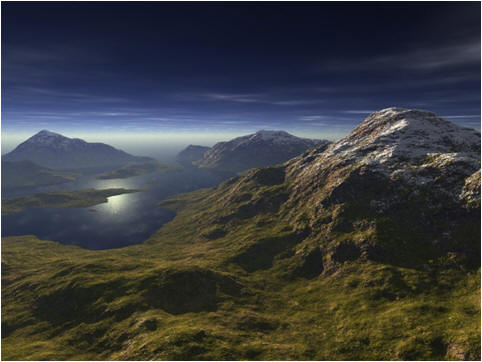
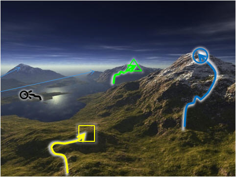
We visualize
fitness landscape of a COP
instance like
this mountain range picture:
*search space (very big), is
visualized as a collection of a lot of points (solutions)
*distance function spatially separates one mountain (solution)
and the other mountains
*objective function determines the height of each mountain
(solution)
*global optima is the highest mountain (solution with the best
objective value)
*local optima is high mountains but not the highest
Notes: This fitness
landscape formulation was proposed by
P. Merz in his
PhD thesis. This definition is slightly different with
the one in
H.H. Hoos and T. Stuetzle's book: SLS:
Foundations and Applications where the fitness landscape is
defined as <search space, neighborhood function, and
objective function>. We do not use neighborhood function as
it will cause our FLST visualization to be unstable
(changing every SLS iteration). |
 |
|
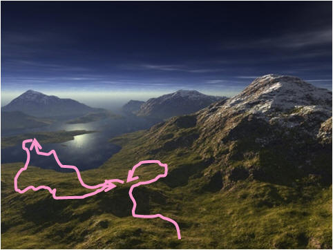
We visualize the search trajectory of
an individual SLS run as a movement of that SLS on the fitness landscape
of the COP instance being attacked. The movement can be due to a local move
within a local neighborhood or a non local move due to strong
diversification mechanism. The objective is to find the global optima: imagine that you are one tiny human in this mountain range and can only
see the surroundings within radius 1 km (local view) and you need to
navigate locally to find the highest mountain.
However, without any 'reference point', it
is quite hard to describe/explain what is going on here (see the
picture on the right and try your best to explain the movement)...
Notes: This search
trajectory formulation is defined in
SLS: Foundations and Applications.
|
 |
|
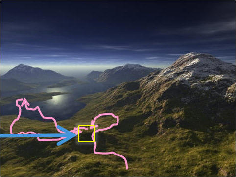
Now suppose that we record the solution
denoted by the yellow rectangle (see the picture on the right).
We can now describe the same search trajectory
above as follows:
"The search trajectory once hits the yellow rectangle solution, then
it moves somewhere
else, then after certain number iterations,
it hits the yellow rectangle solution
again. Is this a solution cycling phenomenon? Is the SLS trapped?".
See that now we can say more things
with the existence of a reference point. |
 |
|
To build the FLST visualization, we gather
a constant amount of high quality (usually local optima), diverse, frequently
visited solutions in the fitness landscape using the SLS algorithms
themselves! We know that we cannot expect to record all
points (exponential space!) therefore we should expect to miss
some good points (look at the small blue arrows pointing at the other two
mountain peaks at the background). Nevertheless, if the
anchor points collected are reasonably good, diverse, and -that is- the
important ones, we can say that we have a
reasonable approximation of the fitness landscape.
In order to collect these points, we run the SLS with different
configurations, with longer run
times, and let it loose.
It will then sample various points in the search space. We then filter
the interesting points which we called: the Anchor Points,
abbreviated as APs. |
 |
|
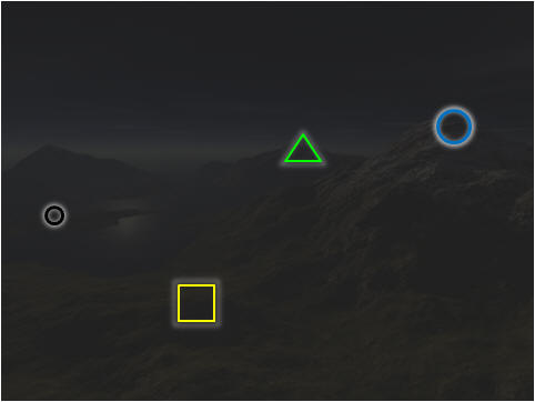
We can also add quality information by labeling these anchor points
with color+shape:
*black
dot-very bad,
*yellow rectangle-bad,
*green triangle-medium,
*blue circle-good.
We use both color and shape as color alone is hard to be
distinguished in black and white scientific papers! Remember
that not all scientific publications out there are in color
at this point of time. |
 |
|
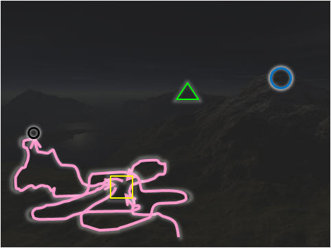
So now, we have this Fitness Landscape
visualization based on these 4 selected APs.
With these APs, we can now describe the search trajectory:
In the picture on the right, the
pink search trajectory encounters
solution cycling in yellow/black (poor) APs.
It fails to reach the
better green/blue (better) APs.
|
 |
|
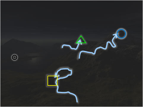
And for this picture on the right, the
blue search trajectory
performs a diversification strategy after hitting an AP (local optima).
From this visualization, we see that it manages to reach the better
green/blue APs
and we can say that it performs better than the
pink search trajectory
above.
This is our proposed FLST
visualization.
If you have any comments, please don't hesitate to email the main
author:
stevenhalim at gmail dot com
|
 |
With FLST visualization,
one can answer these
COP fitness landscape characteristics and SLS behaviors questions (not exhaustive):
The fitness landscape characteristics of
the COP instance:
1. Are the local optima clustered or
spread?
2. Does the fitness landscape smooth or rugged?
3. How many objective value levels in the fitness landscape? is it
discrete or continuous?
4. Are there infeasible regions and where are they located?
The search trajectory behaviors of the SLS
algorithm on a particular COP instance/fitness landscape:
1. Does the SLS behave like as what we intended? How does it make
progress? Does it quickly find the best known solution or wander around in other
regions?
2. How good is the SLS in intensification and diversification?
3. Is there any sign of cycling behavior (search stagnation)?
4. Where in the fitness landscape does the SLS
spend most of its time?
5. How far is the starting/initial/greedy
solution w.r.t the global optima/best known solution?
6. How wide is the SLS coverage?
7. What is the effect of modifying a certain
search parameter/component/strategy w.r.t the SLS behavior?
8. How do two different SLS algorithms (on the same COP fitness
landscape) compare?
Answering these questions can give insights on designing
better performing SLS algorithm to attack the COP at hand.
4. Implementation of FLST visualization in SLS engineering suite: Viz
Parts of this section has
been presented in UIST
2006 and updated in SLS
2007.
In section 3 above, we show the FLST visualization ideas. In this section, we
explain how we implement those ideas in a concrete visualization tool Viz. Viz consists of two main programs: Viz Experiment Wizard (EW) which
executes SLS algorithms and processes the RunLogs and Viz Single
Instance Multiple Runs Analyzer (SIMRA) which displays FLST
visualization and some other statistical information in a user friendly
GUI.
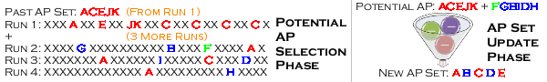
1. Potential AP Selection phase:
Here, Viz EW runs the SLS algorithms (each
with its selected configuration) on the same COP
instance (must be on the same fitness landscape, otherwise the collected points
will be irrelevant with each other) to collect potential local optima points visited by
those SLS. Of course, the SLS must have been augmented with
simple codes to
record search information. We use some of the points found by the SLS algorithms
themselves to visually analyze the SLS performance.
Alternatively, the user can choose to feed Viz EW with RunLog
files generated by their SLS algorithms running in non Windows operating
system. That's it, Viz EW can be set to work with RunLog files only. The non-Windows
users do not need to rewrite or recompile their SLS code in Windows
platform to use this tool. They just need to install Viz on another Windows PC.
e.g. friends'
Windows PC, school's Windows PC, or company's Windows PC, etc and
process the RunLog files there. (however, to fully utilize the benefits of Viz EW, we suggest that
you write a Windows based wrapper code that perform these steps: (1)
login to other OS, (2) executes the SLS algorithm in other OS, and (3)
returns the log files back to Viz EW).
FAQs:
Q: Why do you use SLS algorithms to sample points in the search
space?
A: Obviously, we do not have the time to generate all points using
exact search just to analyze non-exact search trajectories.
The best way is to analyze points visited by the SLS
algorithms itself. Ensure that your SLS algorithm does not stuck
(simply add random restart) so that it samples enough
points. However, even if your SLS algorithm does stuck, this
FLST visualization will show it to you.
Q: Why do you use log file (offline visualization) instead of
real-time visualization?
A: Offline visualization has more advantages. First, we can display the final AP
set so that the visualization is more stable rather than
updating the AP set on the fly. Second, by
communicating via log files, one does not need to depend on
any Operating System. Third, visualization takes
some CPU power to be processed, we simply do not want our
visualization algorithm compete
with the SLS algorithm in terms of CPU resource.
Q: Wait, is
it true that Viz can only analyze 1 (ONE)
single COP instance at one time. Will that be myopic?
A: We agree that analyzing SLS algorithm must be done with
respect to several instances so that our observations are not instance
specific only. Viz is designed to analyze the details of various SLS
runs on a single/1/one COP instance. However, you can still run your SLS algorithm on several training instances
using Viz EW. You will
obviously see different
details from one instance with the other instances but you should have
identify more or less some general characteristics (e.g. all training
instances have "Big Valley" properties, etc).
2. AP Update phase:
In this phase, after the potential APs have been collected, Viz EW filters them and pick a
small number of more diverse and
high quality APs to form an updated AP set. The reason of this step is
simply because we cannot
draw too many points on the screen.
FAQs :
Q: How many points in the screen is 'too many'?
A: As soon as one needs to use zoom in/out, panning
(scroll left/right/up/down), or image distortion (e.g.
fisheye technique), then the points are too many.
Zooming, panning, image distortion, etc decrease the capability of the user in
finding information from visualized data. Therefore, the
number of points is set to be reasonably small, which is currently set
to be min(50,0.5*instance size n).
Q: But, the number of points in the screen can be 'enlarged' if you use
larger monitor, why don't you assume that the end users are using large
monitor?
A: At this point of time, we designed Viz to work under 800*600 monitor
resolution. That gives us 480,000 pixels to play with. Soon, we will
increase Viz default window size to 1024*768, which is about 786,432
pixels, around 1.5 more pixels to work with. However, we cannot keep
enlarging Viz window size as currently the typical monitor resolution is
around [1024*768 .. 1200*800]. We want Viz to work for this kind of
monitor resolution and thus can be used by most people that own a
computer today!
Q: How do you actually filter the points?
A: The actual strategy is a bit too technical and still
under research. In general, we select AP points based on these criteria:
(1). have high quality (randomly selected from the top K% of the
collected points), (2). increase diversity of the AP set (if we already
have good point X in the AP set, we do not include X' which is very
similar to X), (3). have some importance in the SLS runs used to form
the AP set (e.g. the best solution found by the SLS, the most frequently
visited solution, etc).
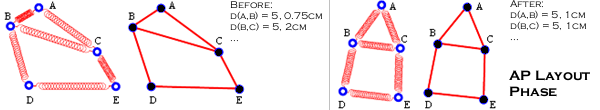
3. AP Layout phase:
After the AP set is selected, Viz layouts the APs in the abstract 2-D space
using a spring model (also
called
force-directed layout algorithms). We measure the distance (bond-number
of different edges,
Hamming-number
of different bits, etc) between APs to set up the spring model. The spring system
will try to stretch and shrink itself into its most natural state
(minimal tension) and that make APs that are close to each other to
appear close in the visualization and vice versa.
We found that presenting the fitness
landscape information in spatial manner like this is quite natural and
easy to
comprehend.
FAQs:
Q: Why use spring model and not any other ways?
A: It is so far the most natural representation that we can
think of. We are also aware of other graph drawing technique like
constraint stress majorization algorithm and will explore other
techniques soon.
Q: What if the distance metric for the solutions in my COP
are not Hamming or bond distance?
A: We are in process of extending the built-in distance
metric inside Viz. Please co-operate with us by e-mailing the main
author: stevenhalim at gmail dot com these information: the COP that you
are planning to attack and the algorithm to compute distance metric that
you think will be suitable for your COP.
4. AP Labeling phase:
After the AP layout phase, we further enhance the fitness landscape presentation by labeling the APs using color and shape labels
as shown in the legend below.
Now with one glance, we know the rough distribution and
quality of the
anchor points.
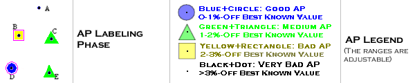
FAQs :
Q: Do you have any particular reason why you choose these
set of colors?
A: The color set is actually taken from the color set used
in geographical map where blue represents deep oceans, green represents
the forests, yellow represents the mountains, and white surroundings
around black dot represents the snowy peaks.
Q: Why do you use double features: shape and color, for the
labels?
A: While color is the best means to group these information, it is quite hard to see in
black and white scientific papers. So we add the shape :)
5. Search Trajectory Layout phase:
Now that we have the abstract 2-D space of
anchor points ready, we can visualize the movements of
the current point/solution (which is actually an N-dimensional combinatorial solution)
of the SLS run as it pass through the COP Fitness Landscape.
We playback the individual SLS run by measuring the distance of the
current solution of an SLS run with the APs. If it is close, we draw a
circle (smaller circle: more similar, larger circle: more different). If
the current solution is nowhere near any of the selected APs, we do not
draw anything (no information can be gained from this iteration). The
movement (appearance and disappearance) of these circles tells us about
the SLS trajectory.
As an example, we explain the interpretation of the search
trajectory visualization of the four runs above (see step 1). The
interpretation depends on the position and quality of APs
visited by the search trajectory. These are the possible interpretations:
Run 1: SLS visits medium quality (green
triangle) APs
and encounter solution cycling issue near AP C. Perhaps AP C is too attractive
even though it is not the best quality (AP D has better quality as
indicated by its
blue circle lable).
Run 2: SLS visits bad region (yellow
rectangle): AP B,
then somewhere near AP C (here we assume that solution F in run 2 is close to
AP C, just to illustrate the drawing of circle with larger diameter
around AP C), and finally arrive at AP A (very bad/black
dot). Perhaps this SLS is not doing a good intensification.
Run 3: SLS starts from a very bad AP A
(black dot), gradually
moves to medium AP C (green triangle), then to good AP D (blue circle).
This SLS behavior is quite okay.
Run 4: The SLS trajectory is not
close to any known AP. It is exploring somewhere else, but definitely
not somewhere near these selected anchor points, it only hits AP A (very
bad/black
dot AP).
FAQs:
Q: Do you know any other ways to visualize search trajectory?
A: To date this is our best way to visualize search
trajectory. We will keep exploring other alternatives.
Q: Do you realize that when two people look at the same FLST
visualization, they may arrive at different interpretations?
A: We agree with that. There may be more than one way to
interpret the visualization and two algorithm designer may design two
different SLS algorithms based on the visualization. Eventually, we just
want improved SLS algorithms. If both interpretations yield
improvements, that is ok.
Q: My SLS is not a trajectory based visualization! I am using population
based algorithm. So how to visualize the 'search trajectory' of a
population?
A: To date, our best way to overcome this situation is by
defining the search trajectory as the movement of the 'best solution
within the population' from one generation to the next... We are
exploring some visualization ideas to better visualize population based
SLS algorithm.
Q: How accurate is
this FLST visualization?
A: The accuracy of FLST visualization is still a research topic.
We know that the accuracy will depends on at least two things: (1). the
number of anchor points that the user wants to display on the screen
(more APs, more layout errors), (2). the way we select AP set (if we
miss important APs, the FLST visualization will be less accurate).
Viz SIMRA, the program that displays this FLST visualization, has few
more features that have not been elaborated. We invite the reader the
visit our Viz version history to appreciate
the development of Viz SIMRA user interface. The GUI are designed with
end user in mind and it boasts the following features: coordinated
visualizations from various angle, visual comparison, animated search
playback, heavy usage of color and highlighting, multiple level of
details, and including some built-in statistical analysis.
This concludes section 4.
5.
The Integrated White and Black Box Approach (IWBBA)
This section has been
presented in CP
2007.
FLST visualization can give us insights of the approximate fitness
landscape structures and SLS behavior. However, while that may give you
insights to design good performing SLS algorithm, it is still not enough if we
want the 'best' performing SLS algorithm for our COP.
We suggest that one combines the strength of the white-box approach with
black-box approach:
1. In white box approach, we analyze our SLS algorithm by means of
statistic or information visualization techniques to gain insights on
how to design better performing SLS algorithm that match the observed
fitness landscape characteristics.
2. In black-box approach, we use a specialized tuning algorithm which
will find the best configuration for our SLS algorithm given the
configuration space and the training set of COP instances. Examples of
such algorithms are:
ParamILS (Hutter et al., 2007),
F-Race (Birattari, 2004),
CALIBRA (Adenso-Diaz and Laguna, 2006).
We invite the reader to
check our results page where we apply this
IWBBA using Viz on real COPs and
real SLS algorithms.
6. References
These basic ideas are explained in more
details in our publications (download the local copy of those papers
here):
-
S. Halim, R. Yap, H.C. Lau. An Integrated White+Black Box Approach for
Designing and Tuning Stochastic Local Search.
In Principles and Practice of Constraint Programming (CP
2007, Providence, Rhode Island, USA, September 23-27, 2007):
332-347
-
S. Halim, R. Yap.
Designing and Tuning SLS through Animation and Graphics: an
Extended Walk-through.
In Engineering Stochastic Local Search Workshop (SLS
2007, Brussels, Belgium, September 6-8, 2007): 16-30
-
S. Halim, R. Yap, H.C. Lau.
Viz: A
Visual Analysis Suite for Explaining Local Search Behavior.
In User Interface System and Technology (UIST
2006, Montreux, Switzerland, October 15-18, 2006): 57-66
|
|
This document, basic_ideas.html, has been accessed 12041 times since 25-May-07 17:48:42 SGT.
This is the 1st time it has been accessed today.
A total of 5393 different hosts have accessed this document in the
last 6182 days; your host, ec2-18-191-21-86.us-east-2.compute.amazonaws.com, has accessed it 1 times.
If you're interested, complete statistics for
this document are also available, including breakdowns by top-level
domain, host name, and date.
|
|
