This web page introduces the numerical algorithms that are frequently used to solve multimedia analysis problems. All of them can be found in Numerical Recipes in C. 

A set of linear equations can be written in the matrix form

A x = b

where A is a m x n matrix of known coefficients, b is a m x 1 matrix (i.e., column vector) of known data, and x is a n x 1 vector of unknown variables.

• If m < n, the equations have no unique solution.
• If m = n and A has an inverse, then a unique solution exists, which can be obtained using methods such as Gauss-Jordan elimination, LU decomposition, singular value decomposition (SVD), etc.
• If m > n, the equations are overconstrained and there may not be an exact solution for x. In this case, we can solve for the x that minimizes the squared error

E ² = ||A x - b||^{2 .}

          That is, perform linear least-squares fitting.

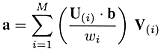
We wish to fit a set of data points (x_i , y_i ) to a linear model such that

y_i = X^T(x_i ) a

where X is a vector of known function and a is a vector of unknown parameters. Let's collect the y_i into a vector b and the X^T(x_i ) into the rows of a matrix A. Then, we have

A a = b .

Least-square fitting looks for the a that minimizes

E ² = ||A a - b||²

This problem can be solved using singular value decomposition (SVD). The SVD of A is

A = U diag(w₁,..., w_n) V^T

and x is given by

a = V diag(1/w₁,..., 1/w_n) U^T b

i.e.,

where U_{( i )} and V_{( i )} are the ith column vectors of U and V.

Note: Least-squares fitting problem is also a minimization problem, that is, to minimize the squared error E ².

Another simple method of solving for a is to compute the pseudo-inverse of A:

a = (A^TA)^-1A^Tb .

When the model y(x; a) to be fitted depends nonlinearly on its parameters a, the Levenberg-Marquardt method can be applied. It combines both gradient (first derivative) method and Hessian (2nd derivative) method.

Here, we are interested in minimizing a function f(x) of multidimensional variable x. The simplest method called gradient descent or steepest descent starts off with x equal to some initial value P(0) and updates P(i) according to the negative gradient of f(P(i)):

where h is a constant update rate. This method is usually not very good except for simple problems. But, it is a simple method.

Another method is to apply Powell's direction set method. It will estimate the gradient using the f supplied by the user, and so does not require the user to supply the gradient information.

Two other families of methods require the user to supply the gradient information. The first family of methods is known as the conjugate gradient methods, and the second family is the variable metric or quasi-Newton methods.

Note: Most optimization algorithms require a good guess for the initial P. The nearer the initial P is to the optimal P, the faster the algorithms converge, and the more accurate is the result.

Given a real, symmetric n x n matrix A, there exist vectors v_i and scalar values l_i such that

A v_i = l_i v_i .

The vectors v_i are called the eigenvectors and the scalars l_i the corresponding eigenvalues of the matrix A. There are many implementations of eigen-decomposition, including one in Numerical Recipes in C.