Understanding Privacy leakage in Machine Learning (Part 1)
Understanding Privacy leakage in Machine Learning (Part 1)
This post assumes the reader has considerable understanding of concepts in probability and differential privacy
Background
Let’s first take a look at some definitions and theorems that would be useful in the analysis presented.
Definition 1: (\((\epsilon,\delta)\) Differential Privacy
then the mechanism \(M\) is said to be \((\epsilon, \delta)\) differentially private.
Lemma 1: (Azuma’s Inequality) Let \(C_1, C_2, ..., C_T\) be real valued random variables such that for every \(t \in [T]\), \(Pr[\lvert C_t \rvert \leq \alpha] = 1\), and for every \((c_1, c_2,...,c_{t-1}) \in Supp(C_1, C_2,...,C_{t-1})\), we have
\[\begin{align} \mathbb{E}[C_t | C_1=c_1, C_2=c_2, ..., C_{t-1}=c_{t-1}] \leq \beta, \end{align}\]then for every \(z \geq 0\), we have
\[\begin{align} Pr\big[ \sum_{t=1}^T C_t \geq T\beta + z\sqrt{T} \cdot \alpha \big] \leq e^{-z^2 / 2}. \end{align}\]Problem Setting
Gradient based empirical risk mimimization algorithms deals with training a model iteratively by updating it’s parameters in a direction that minimizes a target loss objective, typically over a dataset. These learning algorithms are sometimes susceptible to memorizing outlier datapoints
However, privacy analysis of perturbed SGD has been challenging. We don’t really know the output distribution of this algorithm for general loss functions. The approach usually followed therefore is to analyze the privacy leak incurred in releasing the gradients computed at every update step and then compose the guarantees to get the overall bound on privacy leakage for releasing the trained model. This is easier to do because of the simplicity of a singular gradient update step, but also gives loose bounds as the adversary is assumed to be much stronger. The adversary sees not only the output model but also the intermediate (noisy) gradients computed in each step of the update.
To get familiar with the composition theorems in differential privacy, we will analyze the following ML training algorithm.
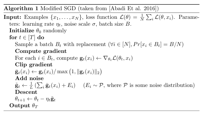
Modifications in Perturbed SGD
Note that the above modified SGD (known as Perturbed SGD) is slightly different in the following aspects:
- Batches are formed by sampling uniformly from dataset with replacement. This is done to make sampling probabilities independent.
- Gradients are Clipped to L2 norm value of 1. This bounds the sensitivity of gradient computation mechanism which helps in privacy loss analysis.
- Some noise is added to the mean gradient before model update. We will analyze the value of the noise variance that guarantees \((\epsilon, \delta)\) differential privacy.
Composition Theorems
Our goal is to compute the total privacy loss of releasing \(T\) gradients updates that results in the output model. We will refer to gradient computation at time \(t\) as mechanism \(M_t\) and the entire training process as mechanism \(M_{1:T}\). Note that the computed gradient at time \(t\) depends on all the gradient outputs at steps \(\langle 1,2,...,t-1 \rangle\) as it is computed on the model parameters that resulted from the previous \(t-1\) updates. In other words, mechanism \(M_{t}\)’s is selected (stochastically of deterministically) based on the outputs \(o_{1:t-1}\). One should therefore understand that the composed mechanism \(M_{1:T}\) is not the same as the product mechanism \(\langle M_1, M_2, ..., M_T \rangle\), as the former doesn’t know the exact mechanisms selected at every step but only the gradients, while the later knows both. However, given the outputs of the first \(T-1\) steps, the exact sequence of \(M_{1:T}\) gets defined and therefore,
\[\begin{align} Pr[M_{1:T}(D) = o_{1:T}] = \prod_{t=1}^T Pr[M_t(D) = o_t \lvert o_{1:t-1}]. \tag{1} \end{align}\]In the context of privacy loss, when the mechanisms at consequent step depends on the previous outputs, privacy leakage can be significantly higher as the sequence of mechanisms themselves could potentially diverge. In differential privacy literature, we have some composition theorems that bounds the privacy leak of mechanism \(M_{1:T}\) by cleverly aggregating losses incurred at every step. We will try to understand these theorems sequentially. First we will look at the weak composition theorem which naively bounds the privacy loss of a mechanisms \(M_{1:T}\). Then, we will try to understand the advanced composition theorem that improves the bounds using Azuma inequality. This bound will further be refined by utilyzing the properties of the noisy distributions’ higher order moments which the advanced composition theorem doesn’t take into account.
Theorem 1: (Composition Theorem) Let \(M_{1:T}\) be a composition of \(T\) mechanisms, such that \(M_t\lvert o_{1:t-1}\) is \((\epsilon_t, \delta_t)\) differentially private for all \(t \in [T]\). Then \(M_{1:T}\) is \((\sum_{t=1}^T \epsilon_t, \sum_{t=1}^T \delta_t)\) differentially private.
Proof: We will prove this for \(T=2\) as using induction, one can then derive the result for \(T > 2\). Let \(D', D'\) be two neighbouring datasets and \(S_1, S_2\) be arbitrary subsets in the range of \(M_1\) and \(M_2\) respectively. Also, let \(\mu(S)\) be defined as follows:
\[\begin{align} \mu(S) = max\big(0, Pr[M_1(D) \in S] - e^\epsilon Pr[M_1(D') \in S] \big). \end{align}\]Since \(M_1\) is \((\epsilon, \delta)\) differentially private, we have \(\mu(S) \leq \delta\) for all subsets of range of \(M_1\). We now prove the theorem as follows:
\[\begin{align*} Pr[M_{1:2}&(D) \in S_1 \times S_2] = \sum_{s_1 \in S_1} Pr[M_{1:2}(D) \in {s_1} \times {S_2}] \\ &= \sum_{s_1 \in S_1} Pr[M_1(D) \in \{s_1\}] \times Pr[M_2(D) \in S_2 \big\lvert s_1] \\ &\leq \sum_{s_1 \in S_1} Pr[M_1(D) \in \{s_1\}] \times (e^{\epsilon_2} Pr[M_2(D') \in S_2 \big\lvert s_1] + \delta_2) \\ &= \sum_{s_1 \in S_1} e^{\epsilon_2} \times Pr[M_1(D) \in \{s_1\}] \times Pr[M_2(D') \in S_2 \big\lvert s_1] \\ &\quad + \delta_2 \times \cancelto{1}{\sum_{s_1 \in S_1}Pr[M_1(D) \in \{s_1\}]} \\ &\leq \delta_2 + e^{\epsilon_2} \sum_{s_1 \in S_1} \big( e^{\epsilon_1} Pr[M_1(D') \in \{s_1\}] + \mu(\{s_1\}) \big) \\ &\quad\quad\quad\quad\quad\quad\quad \times Pr[M_2(D') \in S_2 \big\lvert s_1] \\ &= \delta_2 + e^{\epsilon_1 + \epsilon_2} \sum_{s_1 \in S_1} \big(Pr[M_1(D') \in \{s_1\}] \times Pr[M_2(D') \in S_2 \big\lvert s_1]\big) \\ &\quad + \cancelto{\leq 1 }{e^{\epsilon_2} \times Pr[M_2(D') \in S_2 \big\lvert s_1]} \sum_{s_1 \in S_1} \mu(\{s_1\}) \\ &\leq \delta_2 + \mu(S_1) + e^{2\times\epsilon} \sum_{s_1 \in S_1} e^\epsilon Pr[M_{1:2}(D') \in \{s_1\} \times S_2] \\ &\leq e^{\epsilon_1 + \epsilon_2} Pr[M_{1:2}(D') \in S_1 \times S_2] + \delta_1 + \delta_2 \\ &\tag*{$\blacksquare$} \end{align*}\]The above composition is considered a naive and loose bound because it only relies on the inequality in the definition of \((\epsilon, \delta)\) differential privacy. To understand why this bound is loose, let’s consider an accountant that is tasked with tracking the sequence of privacy losses seen from step \(1\) through \(T\). At every step \(t\), the algorithm stochastically releases an outcome which, by DP assumtion, leaks less than \(\epsilon_t\) in log-likelihood privacy ratio with probability more than \(1 - \delta_t\). The naive accountant exactly allows every step a freedom of \(\delta_t\) probability to leak more than \(\epsilon_t\). Therefore the probability that one or more steps leaks more than their \(\epsilon_t\) qouta becomes \(1 - \prod_{t=1}^T(1 - \delta_t)\) which is less than \(1 - \sum_{t=1}^T \delta_t\). That’s basically how, we get the \((\sum_{t=1}^T \epsilon_t, \sum_{t=1}^T \delta_t)\) differential privacy guarantee. By allowing slightly more freedom to every step can significantly improve the privacy guarantees as seen in the consequent stronger composition theorem.
Theorem 2: (Advanced Composition Theorem) Let \(M_{1:T}\) be a composition of \(T\) mechanisms, such that \(M_t\lvert o_{1:t-1}\) is \((\epsilon, \delta)\) differentially private for all \(t \in [T]\). Then, for all \(\epsilon, \delta, \delta'\), the composed mechanism \(M_{1:T}\) is \((\epsilon', T\delta + \delta')\) differentially private, where
\[\begin{align} \epsilon' = \sqrt{2T\ln(1/\delta')\epsilon} + T\epsilon(e^\epsilon - 1). \tag{2} \end{align}\]Proof: Lets assume that \(D,D'\) are two neigbouring datasets. For any mechanism \(M\), we define the privacy loss at an outcome \(o\) as
\[\begin{align} c(o; M, D, D') \triangleq log \frac{Pr[M(D) = o]}{Pr[M(D') = o]}. \tag{3} \end{align}\]We choose this definition of privacy loss because it is closely related to the \((\epsilon, \delta)\) differential privacy definition. To see this, consider \(B\) to be defined as the following set:
\[\begin{align} B = \{o: Pr[M(D) = o] \geq e^{\epsilon'} Pr[M(D') = o]\}. \tag{4} \end{align}\]Showing that \(M\) is \((\epsilon, \delta)\) differentially private is equivalent to showing that
\[\begin{align} \underset{o \sim M(D)}{Pr} [c(o; M, D, D') \geq \epsilon] \leq \delta. \tag{5} \end{align}\]The reason is due to the following:
\[\begin{align*} Pr[M(D) \in S] &= Pr[M(D) \in S \cap B] + Pr[M(D) \in S \cap B^c] \\ &\leq e^{\epsilon} Pr[M(D') \in S \cap B^c] + Pr[M(D) \in B] \\ &= e^{\epsilon} Pr[M(D') \in S \cap B^c] \\ &\quad + \underset{o \sim M(D)}{Pr} [c(o; M, D, D') \leq \epsilon] \quad\ \ \text{(From (3) and (4))} \\ &\leq e^{\epsilon} Pr[M(D') \in S] + \delta \quad\quad\quad\quad\quad\quad\quad\quad \text{(From (5))} \\ \end{align*}\]Therefore, we will show that (5) is true for mechanism $M_{1:T}$. To do this we will use (1) to break the total privacy loss of \(M_{1:T}\) as the sum of independent privacy loss of every intermediate step t. Then using Azuma’s inequality, for any given \(\delta'\), we will bound the probabily of the total loss exceeding \(\epsilon'\) (defined in (2)) to be less than \(\delta'\).
For an observation \(o_{1:T}\), privacy loss of the composed mechanism \(M_{1:T}\) is given by:
\[\begin{align} c(o_{1:T}; M_{1:T}, D, D') &= log \frac{Pr[M_{1:T}(D) = o_{1:T}]}{Pr[M_{1:T}(D') = o_{1:T}]}\\ &= log \prod_{t=1}^T \frac{Pr[M_t(D) = o_t | o_{1:t-1}]}{Pr[M_t(D') = o_t | o_{1:t-1}]} \tag{From (1)} \\ &= \sum_{t=1}^T log \frac{Pr[M_t(D) = o_t | o_{1:t-1}]}{Pr[M_t(D') = o_t | o_{1:t-1}]} \\ &= \sum_{t=1}^T c(o_t;M_t \lvert o_{1:t-1}, D, D') \tag{From (1)} \\ \end{align}\]Notice that for \(o_{1:T} \sim M_{1:T}(D)\), \(C_t \triangleq c(o_t; M_{1:T} \lvert o_{1:t-1}, D, D')\) are independent random variables \(\forall t \in [T]\). We can therefore bound L.H.S of equation (5) using Azuma’s inequality as follows:
\[\begin{align*} \underset{o \sim M_{1:T}(D)}{Pr} [c(o; M_{1:T}, D, D') \geq \epsilon'] &= Pr[\sum_{t=1}^T C_t \geq \epsilon'] \\ &\quad\quad\quad\quad\quad\quad\quad\text{(Where $\epsilon'$ is given by (2))}\\ &\leq T\delta + \delta' \\ &\quad\quad\quad\quad\quad\quad\quad\text{(By Azuma's Inequality.)} \\ &\text{($\alpha=\epsilon$, $\beta=\epsilon(e^\epsilon - 1)$ and $T\delta + \delta' = e^{-z^2/2}$)} \\ &\tag*{$\blacksquare$} \end{align*}\]So what is the difference between these two composition theorems? For starters, one can see that the \(\delta\) term in composition theorem 2 is weaker than that in theorem 1 (by \(\delta'\) precisely), but the \(\epsilon\) term is considerably smaller. Why are we getting such a big improvement? It’s because the accountant behind advanced composition theorem allows more freedom to every step. Rather than allowing a fixed probability budget of \(\delta\) per step to violate privacy loss bounds, the advanced accountant allows a fixed total budget of \(T\delta + \delta'\) across all steps. This flexibility across steps significantly reduces the privacy loss \(\epsilon'\) that we can promise and is given by equation (2).
Can this bound be improved further? What else can we exploit to get even tighter bounds? It turns out that Azuma’s Inequality used in step (5) above is a bottleneck because it assumes we only know the bound on first moment of the conditional random variables \(C_t \lvert C_{1:t-1} = c_{1:t-1}\). When nothing is known about the individual step mechanisms other than the fact that they are \((\epsilon, \delta)\) differentially private, only a bound on the first moment can be derived from the definition and so the bound from theorem 2 is the best available. However, if there is more knowledge available about the distributions (for instance in the modified SGD above, we know that the distributions are Gaussian), it is possible to derive a tighter bound than what is given by Azuma’s Inequality, and is precisely what we would capitalize in the next composition theorem.
Theorem 3: (Moments’ Accountant Theorem from [Abadi Et al. 2016]) For any mechanism \(M\) and two neighbouring datasets \(D, D'\), let \(\alpha_M\) be defined as the log of the moment generating function for privacy loss random variable \(c(o; M, D, D')\) when \(o \sim M(D)\), i.e.
\[\begin{align} \alpha_M(\lambda; D, D') = log \underset{o \sim M(D)}{\mathbb{E}} \big[exp\big(\lambda c(o; M, D, D')\big) \big], \tag{6} \end{align}\]Then, for any \(\epsilon \geq 0\), the composed mechanism \(M_{1:T}\) is \((\epsilon, \delta)\) differentially private for \(\delta\) that satisfies
\[\begin{align} \delta \geq exp\big(\sum_{t=1}^T \alpha_{M_t \lvert o_{1:t-1}}(\lambda; D, D') - \lambda \epsilon\big) \tag{7} \end{align}\]for all neighbouring \(D, D'\) and some \(\lambda \geq 0\).
Proof: The proof follows the same chain of arguments as the composition theorem 2 but instead of breaking the total privacy loss as a sum of random variables \(\langle C_1, ..., C_T\rangle\), we break the moment generating function of total privacy loss into the sum of a sequence of moment generating functions corresponding to step losses. This is advantageous because the moment generating function can generate all the moments of a random variable and bounds based on it will be tighter than any tail bounding method (such as Azuma’s Inequality) which focuses on a single moment. We show this decomposition as follows:
Consider any pair of neighbouring databases \(D, D'\) and any \(\lambda \geq 0\). Following the definition of \(\alpha\) (defined in (6)) on the composed mechanism \(M_{1:T}\), we have the following decomposition:
\[\begin{align} \alpha_{M_{1:T}}(&\lambda; D, D') = log \underset{o_{1:T} \sim M_{1:T}(D)}{\mathbb{E}} \big[exp(\lambda c(o_{1:T}; M_{1:T}, D, D')) \big] \\ &= log \underset{o_{1:T} \sim M_{1:T}(D)}{\mathbb{E}} \big[exp(\lambda \times \sum_{t=1}^T c(o_t;M_{t} \lvert o_{1:t-1}, D, D'))\big] \\ &\qquad\qquad \text{(Decomposition of total privacy loss like before)} \nonumber \\ &= log \underset{o_{1:T} \sim M_{1:T}(D)}{\mathbb{E}} \big[ \prod_{t=1}^T exp(\lambda \times c(o_t;M_{t} \lvert o_{1:t-1}, D, D'))\big] \\ &= log \prod_{t=1}^T \underset{o_{1:T} \sim M_{1:T}(D)}{\mathbb{E}} \big[exp(\lambda \times \underbrace{c(o_t;M_{t} \lvert o_{1:t-1}, D, D')}_{C_t})\big]\\ &\qquad\qquad\qquad\qquad\qquad\quad\text{(Because $C_t$s are independent)} \nonumber\\ &= \sum_{t=1}^T \alpha_{M_t} \lvert o_{1:t-1}(\lambda; D, D') \qquad\text{(From definition of $\alpha$)}\\ \end{align}\]Using the above decomposition, for any \(\epsilon\), we can bound L.H.S. in (5) for the composed mechanism \(M_{1:T}\) as shown below.
\[\begin{align*} \underset{o_{1:T} \sim M_{1:T}(D)}{Pr} [c(o_{1:T};& M_{1:T}, D, D') \geq \epsilon] \\ &=\underset{o_{1:T} \sim M_{1:T}(D)}{Pr} [exp(\lambda c(o_{1:T}; M_{1:T}, D, D')) \geq \exp(\lambda \epsilon)] \\ &\leq \frac{\underset{o_{1:T} \sim M_{1:T}(D)}{\mathbb{E}} \big[exp(\lambda c(o_{1:T}; M_{1:T}, D, D')) \big]}{exp(\lambda\epsilon)} \\ &\qquad\qquad\qquad\qquad\qquad\qquad\text{(By Markov Inequality)}\\ &= \frac{exp(\alpha_{M_{1:T}}(\lambda; D, D'))}{exp(\lambda \epsilon)} \qquad \text{(From definition of $\alpha$)} \\ &= exp(\sum_{t=1}^T\alpha_{M_t \lvert o_{1:t-1}}(\lambda; D, D') - \lambda\epsilon) \end{align*}\]Therefore, if for all neigbhouring database \(D, D'\), any \(\delta\) that satisfies (7) upperbounds the R.H.S. part above. As we have seen before, the above bound implies \((\epsilon, \delta)\) differential privacy and this completes our proof.
\[\begin{align} &\tag*{$\blacksquare$} \end{align}\]Note that unlike the first two composition theorems, we don’t assume \((\epsilon_t, \delta_t)\) differential privacy of every intermediate mechanism in the composition. Instead, we have a stronger assumption that for each of the intermediate mechanism the moment generating function of it’s privacy loss, i.e. \(\alpha_{M_t}\), is known (or a bound on it is known). The reason this is a stronger assumption because knowing \(\alpha_M\), for a mechanism, one can derive tight differential privacy guarantees for the mechanisms, but the reverse is not possible.
Privacy Bounds for Perturbed SGD
We need one more component to get the privacy guarantee for the perturbed SGD algorithm: DP guarantee of a Gaussian Mechanism. This guarantee would give us the privacy cost incurred for releasing each update step’s noisy gradients to the adversary. We can compose this guarantee across all the steps via various composition theorems discussed to get the total DP guarantee.
Theorem 3: (DP guarantee for a Gaussian Mechanism) Let \(f(\cdot)\) be an arbitrary function with an \(l_2\) sensitivity defined as \(\Delta_2(f) = \underset{D \sim D'}{\max} \Vert f(D) - f(D')\Vert_2\). For \(c^2 > 2 \ln(1.25/\delta)\), the Gaussian Mechanism with parameter \(\sigma^2 ≥ c \Delta_2(f)/\epsilon\) is \((\epsilon,\delta)\)-differentially private.
Based on these three composition theorems, we get the following privacy guarantees:
- From
Naive Composition, perturbed SGD satisfies \((\epsilon,\delta)\)-DP with \(\epsilon \geq \frac{4BT\sqrt{\log T/\delta}}{N\sigma}.\) - From
Advanced Composition,perturbed SGD satisfies \((\epsilon,\delta)\)-DP with \(\epsilon \geq \frac{4B\sqrt{T\log T\log 1/\delta}}{N\sigma}.\) - From
Moments' Accountant, perturbed SGD satisfies \((\epsilon,\delta)\)-DP with \(\epsilon \geq \frac{4B\sqrt{T\log 1/\delta}}{N\sigma}.\)