Auditing ε-DP using Reconstruction Attacks

Synthetic data generators (SDG) offers a powerful way to create realistic datasets that have all of the useful statistical properties of real-world datasets. But, how can we be sure that a generative model isn’t just memorizing and reproducing the sensitive data it was trained on? The most reliable approach is with differential privacy (DP)—a formal guarantee on the SDG that provides a worst-case mathematical bound on the level of information that may be leaked. Ensuring DP almost always requires addition of curated noise somewhere in the generation process followed by a careful pen-and-paper analysis to prove that the DP guarantee holds. For obvious reasons, DP generators are not very popular.

• Deliberate injection of noise is always a concern as doing it right in a way that only minimally affects the utility, only to the extent that is neccesary, is extremely hard.

• A bug in the implementation of a DP algorithm can render the guarantee entirely void. These mistakes happen quite a lot, and may sometimes go undetected for long periods of time.

• On the other hand, DP analysis can often be loose. That is, the pen-and-paper bound grossly overestimates the actual DP parameters. As a result, more than necessary noise gets injected to meet a DP budget, which hurts the utility.

• Many generative approaches have some inherent sources of randomness that may boost the privacy of the generated synthetic data, but these sources often aren’t accounted for in the pen-and-paper analysis.

Privacy auditing is an alternative approach to quantifying privacy risk that works in a way that is opposite to formal DP guarantees. If DP guarantees are theoretical upper bounds, a DP audit gives an empirical lower bound on the level of privacy risk exhibited by an instantiation of an algorithm.

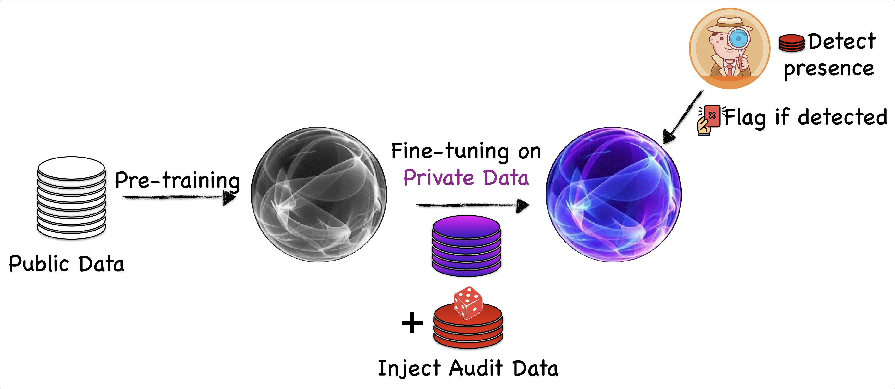
A caricature of how DP auditing for SDG works in general.

In this blog, we describe the in-house DP auditing technique that we developed and actively use at Betterdata. Our DP auditing technique is state-of-the-art and has these three distinguishing characterestics:

• Our audit strategy is built upon reconstruction attacks and not membership-inference attacks.
• We view synthetic data as an unordered reconstruction of the training data, eliminating the need to design custom attacks for SDGs.
• We quantify memorization using nearest-neighbour distances between synthetic and audit data, which resolves the problem of lacking 1-to-1 matches between audit targets and synthetic samples in SDGs.

Our Audit Strategy

At its heart, our method relies on the definition of $\epsilon$-DP. Imagine you have a system that’s supposed to generate synthetic data based on real data, while keeping the original real data private. If this system truly satisfies $\epsilon$-DP, then if someone looks at the synthetic data, they shouldn’t be able to easily figure out what the original, individual real data points were. In other words, their “guess” about the original data after looking at the synthetic data (the posterior distribution) shouldn’t be much different from what they knew beforehand (the prior distribution).

However, if the synthetic data points end up clustering very closely around specific real data points (which we call “audit samples” or “canaries”), it’s like shining a spotlight on those specific real data points. This phenomenon creates “hot-spots” where it’s highly probable that those real examples are located. When this happens, it becomes much easier to pinpoint the original data, which directly violates the $\epsilon$-DP condition. Why? Because the posterior distribution (what you know about the input after seeing the output) is no longer “close” to the prior distribution (what you knew before seeing the output). This closeness is a key requirement for $\epsilon$-DP.

The main finding of our research is that smaller distances between the real audit samples and their closest synthetic counterparts directly indicate a lower privacy guarantee. More precisely, a smaller nearest-neighbor distance means a provably larger lower bound on the system’s true $\epsilon$ value. A larger $\epsilon$ value means less privacy. This conclusion is reached with a high level of statistical confidence.

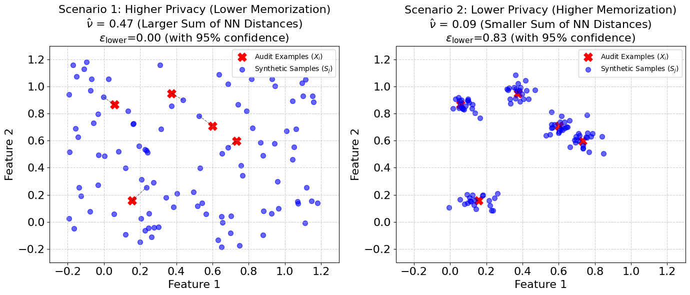
Smaller sum of nearest-neighbor distances ($\hat\nu$) implies provably larger lower bounds on the model’s true $\epsilon$ value.

Procedure. Our audit process is designed to check the differential privacy of the entire system that transforms real data into synthetic data. It treats this system, referred to as algorithm $\mathcal{A}$, as a black-box. This means it doesn’t need to know the inner workings of the generative system. It just observes what goes in and what comes out. The algorithm $\mathcal{A}$ takes a set of $m$ “audit examples” as input and produces $n$ synthetic data points as output. It’s important to note that our audit can be done in a single run, just like the work by Steinke et al, 2023 (which uses membership-inference attack).

\begin{algorithm}
\caption{$\epsilon$-DP Auditor using nearest-neighbour distance sum}
\begin{algorithmic}
\REQUIRE Algorithm $\mathcal{A}$ to audit, number of audit examples $m$, number of synthetic samples $n$, dimension of feature vectors $d$, significance level $\beta$.
\STATE Uniformly sample audit targets $\mathbf{X} = (X_1, \cdots, X_m) \leftarrow^\$ [0,1]^{d \times m}$
\STATE Generate synthetic samples $(S_1, \cdots, S_n) \leftarrow^\$ \mathcal{A}(\mathbf{X})$
\STATE Initialize $\hat\nu \leftarrow 0$
\FOR{$i=1$ {\bfseries to} $m$}
\STATE $\hat\nu \leftarrow \hat\nu + \inf_{j \in [n]} \Vert X_i - S_j \Vert_2$
\ENDFOR
\STATE \textbf{return} $\epsilon_\mathrm{lower} \leftarrow \max \left\{0, \log\left(\frac{\Gamma(d/2)}{\Gamma(d)}\cdot \frac{\sqrt[m]{\beta \cdot (md)!}}{2\pi^{d/2}n\cdot\hat\nu^d }\right) \right\}$
\end{algorithmic}
\end{algorithm}

Here’s a step-by-step explanation of our auditin procedure:

1. Sampling Audit Examples (Canaries): The first step involves uniformly selecting $m$ data points. These points, called audit examples or canaries, are chosen from a $d$-dimensional “hypercube”. This hypercube is defined as a space where all coordinates are between 0 and 1, and it has a unit volume. While for convenience, we set one corner of this hypercube at the origin, it can conceptually be anywhere in the $d$-dimensional space. These audit examples are the specific data points that the audit will try to detect in the synthetic output.

2. Training the Generative Model: These audit examples, sometimes along with a real training dataset (which is considered fixed and “hardcoded” into the algorithm), are then used to train the generative model, which is the usual process of creating a model that can produce synthetic data.

3. Generating Synthetic Samples: After the generative model is trained, it produces $n$ synthetic feature vectors. Optionally, if it’s computationally feasible, these synthetic samples can be constrained to also fall within the same $d$-dimensional hypercube as the audit examples. This is done through “rejection sampling,” which basically means if a generated sample falls outside the hypercube, it’s discarded and a new one is generated until it falls within the desired range. This restriction can improve the audit’s performance.

4. Measuring Memorization (Nearest-Neighbor Distance): This is a crucial step. For each of the $m$ audit examples, the audit finds its nearest neighbor among all the $n$ synthetic examples. The “distance” here is the standard Euclidean distance, which is also known as the Distance to Closest Record (DCR) in the synthetic-generation literature. Once all these nearest distances are found (one for each audit example), they are summed up to get a value called $\hat\nu$. This value, $\hat\nu$, acts as a proxy for how much the generative model has “memorized” the original audit examples. A smaller $\hat\nu$ suggests more memorization.

5. Estimating the Privacy Lower Bound: In the final phase, the calculated $\hat\nu$ value is used to estimate a lower bound on the true $\epsilon$ value of the system’s differential privacy. This lower bound is denoted as $\epsilon_{\mathrm{lower}}$. This means that the system’s actual $\epsilon$ value is guaranteed to be at least $\epsilon_{\mathrm{lower}}$ with certain statistical significance. That is, the calculation considers a “significance level” $\beta$, which basically determines the confidence of the lower bound holding. For example, if $\beta = 0.05$, it means there’s a 95% confidence that the true $\epsilon$ is at least $\epsilon_{\mathrm{lower}}$.

In essence, our audit introduces “canaries” (audit examples) into the system and then checks if these canaries are “visible” in the synthetic output. If they are too visible (i.e., synthetic data clusters too closely around them), it’s a strong indication that the system is not as differentially private as it claims, and the audit provides a quantifiable lower bound on how much privacy is actually being lost. Algorithm 1 describes our approach.

Main Theoretical Result

Let’s dive into the mathematical backbone that allows us to convert that “memorization” measurement, $\hat\nu$, into a concrete privacy estimate. The following main result enables this conversion.

This theorem provides a rigorous mathematical relationship between the observed nearest-neighbor distance sum and the differential privacy guarantee. It states that if a synthetic data generation algorithm $\mathcal{A}$ truly satisfies $\epsilon$-differential privacy, then there’s a limit to how “close” the synthetic samples can get to the original audit examples. Specifically, if we uniformly pick $m$ audit examples ($\mathbf{X}$) and then generate $n$ synthetic samples ($\mathbf{S}$) using $\mathcal{A}$, the probability of the sum of the nearest-neighbor distances ($\hat\nu$) being less than or equal to some constant is bounded. This constant is a formula of the significance threshold ($\beta$), the number of audit examples ($m$), synthetic samples ($n$), the dimension of the data ($d$), and importantly, the privacy parameter $\epsilon$.

To put it more simply, this theorem provides a way to formally test the hypothesis: “Algorithm $\mathcal{A}$ is $\epsilon$-DP.” If we observe a value for $\hat\nu$ that is smaller than this calculated threshold, we can confidently reject the claim that the algorithm $\mathcal{A}$ satisfies $\epsilon$-DP. The p-value of the hypothesis test, which represents the probability of incorrectly rejecting the null hypothesis (i.e., concluding it’s not $\epsilon$-DP when it actually is), is determined by our chosen significance level $\beta$. So, if we choose a $\beta$ of, say, 0.05, we have only a 5% chance of being wrong when we reject the claim.

Our auditor, as presented in Algorithm 1, leverages this hypothesis test to estimate a lower bound on the true $\epsilon$-DP parameter of the algorithm $\mathcal{A}$. The core idea is this: say we observe a specific value of $\hat\nu$ by running the audit. Then, we look at all possible $\epsilon$ values. For each $\epsilon$, if our observed $\hat\nu$ exceeds the threshold constant for that particular $\epsilon$, it means that it’s highly unlikely that the algorithm is actually $\epsilon$-DP for that $\epsilon$. Therefore, we can confidently reject the null hypothesis for that specific $\epsilon$. The maximum $\epsilon$ for which we can confidently reject the null hypothesis becomes our $\epsilon_{\text{lower}}$, which serves as a lower bound estimate for the algorithm’s true privacy parameter. And the beauty of this approach is that we can guarantee this estimate holds with a high probability (at least $1-\beta$).

This means we’re not just saying “it’s not private enough,” but we’re also providing a numerical estimate of how much privacy is likely being violated, with a clear statistical confidence level. This makes our audit a powerful tool for assessing and verifying the differential privacy guarantees of generative mechanisms. The following figure visually demonstrates our auditing technique when applied to a Gaussian Mixture Model (GMM).

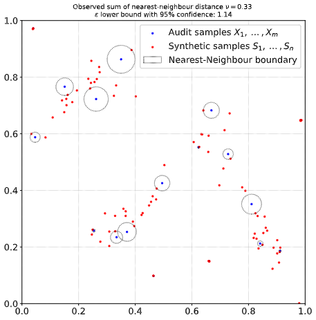
Audit visualization in 2 dimensions. Audit dataset $\mathbf{X}$ consists of $m=20$ uniformly random points. We trained a Gaussian Mixture model with 8 components on $\mathbf{X}$ and generate synthetic dataset $\mathbf{S}$ containing $n=50$ samples.

Problem with Membership-Inference Attacks

Almost all the other DP auditing techniques in literature rely exclusively on membership-inference attacks (MIA). We discovered that MIAs have a serious drawback when it comes to DP auditing. By definition, if a algorithm $\mathcal{A}$ satisfies $\epsilon$-DP, then for all neighbouring datasets $D_0$ and $D_1$ that differ in a single entry and for all sets $S$ in the output domain,

So if the odds of a target being or not being in the input is fifty-fifty, the probability that a membership test that predicts IN or OUT based on whether the output $Y$ lies in some set $S$ is bounded if the algorithm is $\epsilon$-DP.

Even if a membership-inference attack succeeds on a target with a \(100\%\) accuracy across 1 million independent runs, the largest lower-bound on the DP parameter we can infer with a $95\%$ statistical confidence is only $\epsilon_\mathrm{lower} 12.71$. This is because for $\epsilon = 12.71$, the probability of a single membership-inference succeeding in the worst-case is $\frac{1}{e^{-\epsilon} + 1} \approx 0.999997$. Since this probability is extremely close to one, it would take a million consecutively correct membership-inference guesses for there to be a significant enough evidence that the DP parameter $\epsilon = 12.71$ is unlikely to hold (i.e., the p-value for the null-hypothesis that $\epsilon$-DP holds with $\epsilon = 12.71$ holds is $\beta = 0.999997^{1000000} < 0.05$).

Why are reconstruction attacks are superior? The reason why MIAs have such an unreasonable sample complexity is because they test for a single bit at a time—whether the target was included in the training data or not? In contrast, reconstruction attacks attempts to predict all the bits that make up a target, which is significantly better for DP audits. To contextualize, our main result shows that for just $m=n=10$ audit and synthetic samples in $d=10$ dimensions, a nearest-neighbor distance sum $\hat\nu \leq 1$ yields $\epsilon_\mathrm{lower} = 17.34$, $\hat\nu \leq 0.1$ yields $\epsilon_\mathrm{lower} = 40.36$, and $\hat\nu \leq 0.01$ yields $\epsilon_\mathrm{lower} = 63.39$ with $99.9\%$ confidence ($\beta = 0.001$). In fact, as the nearest-neighbour distance sum goes to zero, the lower bound $\epsilon_\mathrm{lower}$ goes to infinity. That is why reconstruction attacks are a whole lot better than membership-inference attacks when it comes to privacy auditing, especially for synthetic data generators.

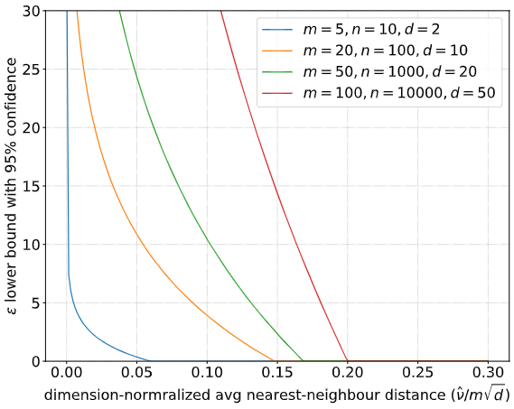
Comparision of $\epsilon_\mathrm{lower}$ derived from our audit algorithm as the dimension-normalized avgerage nearest-neighbor distance metric ($\hat\nu / m\sqrt{d}$) changes for different choices of parameters $(m,n,d)$.

Numerically Stable Implementation

Following codeblock contains an implementation of our DP audit computation. Given an observation of the nearest-neighbor distance sum $\hat\nu$, the first method computes the p-value for a choice of $\epsilon$ and the second method computes the $\epsilon_\mathrm{lower}$ for a choice of significance threshold $\beta$ of the p-value.

import numpy as np
from scipy.special import gammaln

# m = number of audit example vectors
# n = number of synthetic sample vectors
# d = dimension of audit and synthetic feature vectors
# v = sum of Euclidean distances between audit examples and NN synthetic samples
# eps = DP guarantee of null hypothesis
# output: p-value = probability of <=v NN distance sum under null hypothesis
def get_pvalue(m, n, d, v, eps):
    assert v > 0
    assert eps >= 0
    log_gamma_term = gammaln(d) - gammaln(d / 2)
    log_md_factorial = gammaln(m * d + 1)
    log_base_terms = np.log(2) + (d / 2) * np.log(np.pi) + np.log(n) + log_gamma_term
    log_p_value = -log_md_factorial + m * (log_base_terms + eps + d * np.log(v))
    p_value = np.exp(log_p_value)
    return np.minimum(p_value, 1)

# m = number of audit example vectors
# n = number of synthetic sample vectors
# d = dimension of audit and synthetic feature vectors
# v = sum of Euclidean distances between audit examples and NN synthetic samples
# p = 1-confidence e.g. p=0.05 corresponds to 95%
# output: lower bound on eps i.e. algorithm is not eps-DP
def get_epslb(m, n, d, v, p):
    assert v > 0
    assert p > 0
    log_gamma_term = gammaln(d/2) - gammaln(d)
    log_md_factorial = gammaln(m * d + 1)
    log_top_terms = (np.log(p) + log_md_factorial) / m
    log_bottom_terms = np.log(2) + (d / 2) * np.log(np.pi) + np.log(n) + d * np.log(v)
    eps_lower = log_gamma_term + log_top_terms - log_bottom_terms
    return np.maximum(0,eps_lower)