Figure 1. Candles
Important: Please read Lab Guidelines before you continue.
This lab contains 4 exercises. You are required to do the first 3 exercises. Exercise #4 is for your own practice and it will not be graded; it will not be graded by CodeCrunch as well as it involves random numbers.
To receive the attempt mark for this lab assignment, you must submit all 3 programs and get a passing feedback mark for each of the program.
The maximum number of submissions for each exercise is 12.
Please do not use features such as arrays, pointers and recursion
which are not yet covered in class.
In general, for all lab exercises, do not use features not covered yet. When in doubt,
please raise them on IVLE forum or with your DL.
If you have any questions on the task statements, you may post your queries on the relevant IVLE discussion forum. However, do not post your programs (partial or complete) on the forum before the deadline!
Please be reminded that lab assignments must be done in your own effort.
Important notes applicable to all exercises here:
Alexandra has n candles. He burns them one at a time and carefully collects all unburnt residual wax. Out of the residual wax of exactly k (where k > 1) candles, he can roll out a new candle.
Write a program candles.c to help Alexandra find out how many candles he can burn in total, given two positive integers n and k.
The output should print the total number of candles he can burn.
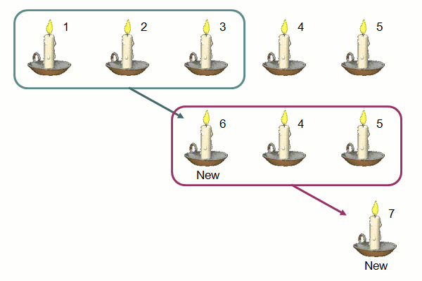
The diagram below illustrates the case of n = 5 and k = 3. After burning the first 3 candles, Alexandra has enough residual wax to roll out the 6th candle. After burning this new candle with candles 4 and 5, he has enough residual wax to roll out the 7th candle. Burning the 7th candle would not result in enough residual wax to roll out anymore new candle. Therefore, in total he can burn 7 candles.
Figure 1. Candles
Sample run using interactive input (user's input shown in blue; output shown in bold purple). Note that the first two lines (in green below) are commands issued to compile and run your program on UNIX.
Sample run #1:
$ gcc -Wall candles.c -o candles
$ candles
Enter number of candles and
number of residuals to make a new candle: 5 3
Total candles burnt = 7
Sample run #2:
Enter number of candles and
number of residuals to make a new candle: 100 7
Total candles burnt = 116
The time here is an estimate of how much time we expect you to spend on this exercise. If you need to spend way more time than this, it is an indication that some help might be needed.
(This is a question in PE1 of AY2013/14 Semester 1. See PE page)
In mathematics, a square number is an integer that is the square of a positive integer. Examples are 9 (= 3 × 3), 4 (= 2 × 2), and 1 (= 1 × 1). 1 is the smallest square number.
On the other hand, a square-free integer is a positive integer divisible by NO square number, except 1. For instance,
The first 10 square-free integers are: 1, 2, 3, 5, 6, 7, 10 ,11, 13, and 14.
Write a program square_free.c to read 4 positive integers in the following sequence: lower1, upper1, lower2, upper2, compute the number of square-free integers in two ranges [lower1, upper1] (both inclusive) and [lower2, upper2] (both inclusive), compare and report which range has more square-free integers.
You may assume that: 1 ≤ lower1 ≤ upper1, and 1 ≤ lower2 ≤ upper2.
No input validation is needed.
For example, in sample run #1 below, range [1, 5] contains 4 square-free integers while range [5, 9] contains 3 square-free integers. Therefore your program should print out:
Range [1,5] has more square-free numbers: 4
Modular design makes your coding easier. Besides the main() function, your program must contain at least another function (of your own choice) to compute some results.
Use the skeleton program given to you. Check sample runs for input and output format.
Sample runs using interactive input (user's input shown in blue; output shown in bold purple). Note that the first two lines (in green below) are commands issued to compile and run your program on UNIX.
Sample run #1:
$ gcc -Wall square_free.c -o square_free
$ square_free
Enter four positive integers: 1 5 5 9
Range [1, 5] has more square-free numbers: 4
Sample run #2:
Enter four positive integers: 1 8 2 10
Both ranges have the same number of square-free numbers: 6
The time here is an estimate of how much time we expect you to spend on this exercise. If you need to spend way more time than this, it is an indication that some help might be needed.
Numerical analysis is an important area in computing. One simple numerical method we shall study here is the Bisection method, which computes the root of a continuous function. The root, r, of a function f is a value such that f(r) = 0.
How does bisection method work? It is best explained with an example. Given this polynomial function p(x) = x3 + 2x2 + 5, we need to first provide two endpoints a and b such that the signs of p(a) and p(b) are different. For example, let a=-3 (hence p(a)=-4) and b=0 (hence p(b)=5).
The principle is that, the root of the polynomial (that is, the value r where p(r) = 0) must lie somewhere between a and b. So for the above polynomial, the root r must lie somewhere between -3 and 0, because p(-3) and p(0) have opposite signs. (NOT because -3 and 0 have opposite signs!)
This is achieved as follows. The bisection method finds the midpoint m of the two endpoints a and b, and depending on the sign of p(m) (the function value at m), it replaces either a or b with m (so m now becomes one of the two endpoints). It repeats this process and stops when one of the following two events happens:
Figure 2 below shows the two endpoints a (-3) and b (0), their midpoint m (-1.5), and the function values at these 3 points: p(a) = -4, p(b) = 5, p(m) = 6.125.
Since p(m) has the same sign as p(b) (both values are positive), this means that m will replace b in the next iteration.
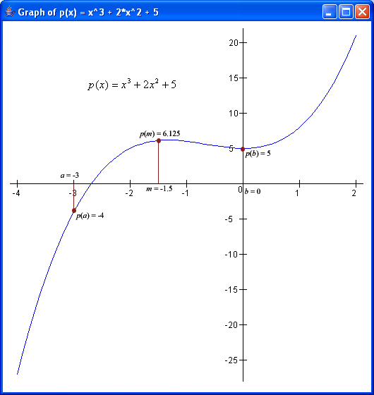
Figure 2. Graph of p(x)
= x3 + 2x2 + 5
The following table illustrates the iterations in the process. The end-point that is replaced by the mid-point value computed in the previous iteration is highlighted in pink background.
| iteration | endpoint a | endpoint b | midpoint m | function value p(a) | function value p(b) | function value p(m) |
| 1 | -3.000000 | 0.000000 | -1.500000 | -4.000000 | 5.000000 | 6.125000 |
| 2 | -3.000000 | -1.500000 | -2.250000 | -4.000000 | 6.125000 | 3.734375 |
| 3 | -3.000000 | -2.250000 | -2.625000 | -4.000000 | 3.734375 | 0.693359 |
| 4 | -3.000000 | -2.625000 | -2.812500 | -4.000000 | 0.693359 | -1.427002 |
| 5 | -2.812500 | -2.625000 | -2.718750 | -1.427002 | 0.693359 | -0.312714 |
| 6 | -2.718750 | -2.625000 | -2.671875 | -0.312714 | 0.693359 | 0.203541 |
| 7 | -2.718750 | -2.671875 | -2.695312 | -0.312714 | 0.203541 | -0.051243 |
| 8 | -2.695312 | -2.671875 | -2.683594 | -0.051243 | 0.203541 | 0.076980 |
| 9 | -2.695312 | -2.683594 | -2.689453 | -0.051243 | 0.076980 | 0.013077 |
| 10 | -2.695312 | -2.689453 | -2.692383 | -0.051243 | 0.013077 | -0.019031 |
| 11 | -2.692383 | -2.689453 | -2.690918 | -0.019031 | 0.013077 | -0.002964 |
| 12 | -2.690918 | -2.689453 | -2.690186 | -0.002964 | 0.013077 | 0.005059 |
| 13 | -2.690918 | -2.690186 | -2.690552 | -0.002964 | 0.005059 | 0.001048 |
| 14 | -2.690918 | -2.690552 | -2.690735 | -0.002964 | 0.001048 | -0.000958 |
| 15 | -2.690735 | -2.690552 | -2.690643 | -0.000958 | 0.001048 | 0.000045 |
| 16 | -2.690735 | -2.690643 | -2.690689 | -0.000958 | 0.000045 | -0.000456 |
Hence the root of the above polynomial is -2.690689 (because the difference between a and b in the last iteration is smaller than the threshold 0.0001), and the function value at that point is -0.000456, close enough to zero.
(Some animations on the bisection method can be found on this website: Bisection method. Look at the first one.)
Write a program bisection.c that asks the user to enter the integer coefficients (c3, c2, c1, c0) for a polynomial of degree 3: c3*x3 + c2*x2 + c1*x + c0. It then asks for the two endpoints, which are real numbers. You may assume that the user enters a continuous function that has a real root. You may use the double data types for real numbers. To simplify matters, you may also assume that the two endpoints the user entered have function values that are opposite in signs.
Your program should have a function double polynomial(double, int, int, int, int) to compute the polynomial function value. This is mandatory.
In the output, real numbers are to be displayed accurate to 6 decimal digits (see output in sample runs below).
Sample run using interactive input (user's input shown in blue; output shown in bold purple). Note that the first two lines (in green below) are commands issued to compile and run your program on UNIX.
Only the last 2 lines shown in bold purple are what your program needs to produce. The iterations are shown here for your own checking only.
The sample run below shows the output for the above example. Note that the iterations end when the difference of the two endpoints is less than 0.0001, and the result (root) is the midpoint of these two endpoints.
$ gcc -Wall bisection.c -o bisection
$ bisection
Enter coefficients (c3,c2,c1,c0) of polynomial: 1 2 0 5
Enter endpoints a and b: -3 0
#1: a = -3.000000; b = 0.000000; m = -1.500000
     p(a) = -4.000000; p(b) = 5.000000; p(m) = 6.125000
#2: a = -3.000000; b = -1.500000; m = -2.250000
     p(a) = -4.000000; p(b) = 6.125000; p(m) = 3.734375
#3: a = -3.000000; b = -2.250000; m = -2.625000
     p(a) = -4.000000; p(b) = 3.734375; p(m) = 0.693359
#4: a = -3.000000; b = -2.625000; m = -2.812500
     p(a) = -4.000000; p(b) = 0.693359; p(m) = -1.427002
#5: a = -2.812500; b = -2.625000; m = -2.718750
     p(a) = -1.427002; p(b) = 0.693359; p(m) = -0.312714
(... omitted for brevity ...)
#15: a = -2.690735; b = -2.690552; m = -2.690643
     p(a) = -0.000958; p(b) = 0.001048; p(m) = 0.000045
#16: a = -2.690735; b = -2.690643; m = -2.690689
     p(a) = -0.000958; p(b) = 0.000045; p(m) = -0.000456
root = -2.690689
p(root) = -0.000456
The second sample run below shows how to find the square root of 5. For polynomial where there are more than one real root, only one root needs to be reported.
$ bisection
Enter coefficients (c3,c2,c1,c0) of polynomial: 0 1 0 -5
Enter endpoints a and b: 1.0 3.0
#1: a = 1.000000; b = 3.000000; m = 2.000000
     p(a) = -4.000000; p(b) = 4.000000; p(m) = -1.000000
#2: a = 2.000000; b = 3.000000; m = 2.500000
     p(a) = -1.000000; p(b) = 4.000000; p(m) = 1.250000
(... omitted for brevity ...)
#16: a = 2.236023; b = 2.236084; m = 2.236053
     p(a) = -0.000201; p(b) = 0.000072; p(m) = -0.000065
root = 2.236053
p(root) = -0.000065
The third sample run below shows how to find the root of the function 2x2 - 3x. Since the midpoint of the given endpoints a and b is 1.5 which is the root of the function, the loop ends after the first iteration.
$ bisection
Enter coefficients (c3,c2,c1,c0) of polynomial: 0 2 -3 0
Enter endpoints a and b: 0.5 2.5
#1: a = 0.500000; b = 2.500000; m = 1.500000
     p(a) = -1.000000; p(b) = 5.000000; p(m) = 0.000000
root = 1.500000
p(root) = 0.000000
The time here is an estimate of how much time we expect you to spend on this exercise. If you need to spend way more time than this, it is an indication that some help might be needed.
This exercise might take you a lot of time testing and debugging.
p, or pi, is a well-known constant 3.14159265..., which is the ratio of a circle's circumference to its diameter.
Consider the unit circle which, in cartesian coordinates, is defined by the equation x*x + y*y = 1. Its area is pi, and hence the area of the part of the unit circle that lies in the first quadrant is pi/4.
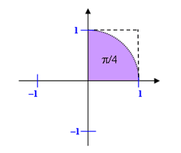
Figure 3.
Imagine that you throw darts at random at the unit square (in the first quadrant) so that the darts land randomly on (x, y) coordinates satisfying 0 ≤ x ≤ 1 and 0 ≤ y ≤ 1. Some of these darts will land inside the unit circle's quadrant. As shown in Figure 3 above, the unit square is the square box which contains the unit circle's quadrant (the purple-shaded region).
Since the unit circle's quadrant has area pi/4 and the unit square has area 1, if you program it such that the darts always land within the unit square, then the proportion of darts you randonly throw that land in the unit circle's quadrant will be approximately pi/4.
(How do you determine if a dart lands inside the unit circle's quadrant?)
Write a program montecarlo.c that asks the user to enter the number of darts to throw. Pass this value to a function throwDarts(int). This is a mandatory function.
In the function, generate the appropriate random numbers to simulate the throwing of darts. Calculate the number of darts that land inside the unit circle's quadrant. (Consider the dart to have landed inside if x2 + y2 ≤ 1, i.e. including the unlikely event that it lands exactly on the boundary of the unit circle's quadrant.) Return this number back to the caller, which then computes the approximate value of pi.
It is reasonable to expect that the more darts we throw, the more accurately the computed value of pi approximates the real value of p.
Your program should output the number of darts that landed inside the unit circle's quadrant, and the value of pi computed correct to 4 decimal places.
Sample run using interactive input (user's input shown in blue; output shown in bold purple). Note that the first two lines (in green below) are commands issued to compile and run your program on UNIX.
Sample run #1:
$ gcc -Wall montecarlo.c -o montecarlo
$ montecarlo
How many darts? 5000
Darts landed inside unit circle's quadrant = 3934
Approximated pi = 3.1472
Sample run #2:
$ montecarlo
How many darts? 90000000
Darts landed inside unit circle's quadrant = 70686491
Approximated pi = 3.1416
The time here is an estimate of how much time we expect you to spend on this exercise. If you need to spend way more time than this, it is an indication that some help might be needed.
The deadline for submitting all programs is 18 September 2017, Monday, 5pm. Late submission will NOT be accepted.