Parallel Banding Algorithm to Compute Exact Distance Transform with the GPU

Thanh-Tung Cao, Ke Tang, Anis Mohamed, and Tiow-Seng Tan

{ caothanh | tangke | tants }@comp.nus.edu.sg, mohd.anis@gmail.com

School of Computing

National University of Singapore


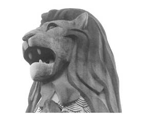
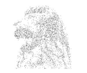
Original Image	Sampled Image	Result by CVD

Abstract

We propose a Parallel Banding Algorithm (PBA) on the GPU to compute the exact Euclidean Distance Transform (EDT) for a binary image in 2D and higher dimensions. Partitioning the image into small bands to process and then merging them concurrently, PBA computes the exact EDT with optimal linear total work, high level of parallelism and a good memory access pattern. This work is the first attempt to exploit the enormous power of the GPU in computing the exact EDT, while prior works are only on approximation. Compared to these other algorithms in our experiments, our exact algorithm is still a few times faster in 2D and 3D for most input sizes. We illustrate the use of our algorithm in applications such as computing the Euclidean skeleton using the integer medial axis transform, performing morphological operations of 3D volumetric data, and constructing 2D weighted centroidal Voronoi diagrams.

CR Categories: I.3.1 [Computer Graphics]: Hardware Architecture - Graphics Processors; I.3.5 [Computer Graphics]: Computational Geometry and Object Modeling - Geometric Algorithms.

Keywords: Digital geometry, Interactive application, Programmable graphics hardware.

Paper in The Proceedings of ACM SIGGRAPH Symposium on Interactive 3D Graphics and Games (I3D 2010), Maryland, USA, 19–21 February, 2010, pp. 83–90.

Video: click here to download the video clip (58M).

Dated: 10 Jan 2010, 27 Jan 2010, 4 March 2010, 8 Aug 2019

©NUS

Addendum: After A Decade

Jiaqi Zheng and Tiow-Seng Tan

orzzzjq@gmail.com, tants@comp.nus.edu.sg

Over the past 10 years, many researchers have tried our software and provided us some feedback. We read our source code again and put in some efforts to improve its performance. To date, we have created a new version, termed PBA⁺, and it is made available for download at here.

This addendum records the following about PBA and PBA⁺:

Review of the PBA code
Improvement of PBA to PBA⁺
New Experiments on PBA and PBA⁺

Review of the PBA code

Let’s first review PBA and its source codes to better prepare ourselves to understand the subsequent content.

The PBA source codes use two transposes in both 2D and 3D version. This is so that threads can deal with the data column by column to coalesce memory loads and stores issued by threads of a warp into as few transactions as possible to minimize DRAM bandwidth. This is very helpful to improve the GPU performance, while the transpose operation scale up very well on modern GPUs.
The PBA paper indicated that one can use a parallel prefix approach to propagate the information between the first and the last pixels of all bands. However, the source codes use two for-loops to achieve this propagation of information. Though the complexity of the parallel prefix method is $O(log\space m_1)$ and the complexity of the for-loops is $O(m_1)$, experiments show that, in most cases, parallel prefix is not better than the for-loops. This is because all suitable values of $m_1$ are small and the for-loops thus is still fast with a single CUDA kernel call to complete. In contrast, the parallel prefix method needs to invoke CUDA kernel call many times and thus not necessarily faster than the single call for the for-loop.

There are 3 important parameters $m_1$, $m_2$ and $m_3$ in the 3 phases of PBA respectively. The performance can be affected by the choice of these parameters. With the development of the graphics cards, the optimal values for these parameters also changed. We did some experiments to determine their appropriate values on different GPUs. Our findings are as shown in Table 1 to serve as reference when using our source codes.

Table 1. Appropriate parameters of PBA on different GPUs

Texture Size	GTX 1070			GTX 980Ti			GTX 1080Ti
Texture Size	$m_1$	$m_2$	$m_3$	$m_1$	$m_2$	$m_3$	$m_1$	$m_2$	$m_3$
$512^2$	16	16	8	16	16	16	16	32	16
$1024^2$	16	32	8	16	16	8	16	32	16
$2048^2$	16	32	8	16	16	8	32	32	16
$4096^2$	32	32	4	32	16	4	64	32	8
$8192^2$	32	32	4	32	32	4	128	32	4
$64^3$	1	1	2	1	1	2	1	1	4
$128^3$	1	1	2	1	1	2	1	1	2
$256^3$	1	1	2	1	1	2	1	1	2
$512^3$	1	1	2	1	1	2	1	1	2

Improvement of PBA to PBA⁺

We discuss here how we improve PBA.

We improved both the 2D and 3D version of PBA. In the old version, we utilized the texture cache for better performance, but because of the performance of global memory improved and our good memory access pattern, there is actually no difference between global memory and texture memory in PBA on modern GPUs. In the new version PBA⁺, we only use global memory to utilize the memory for larger input.
The PBA source codes handle the two transposes as two separate steps. We managed to merge these transposes into the working of Phase 1 and Phase 3 respectively. Specifically, in Phase 1 and Phase 3, we first store the result of the corresponding phase in a square shared memory, and then write it into the corresponding transposed position of global memory, as shown in Figure 1. Assume there are $k$ thread within a CUDA block and the size of a shared memory $\mathbb{S}$ is $k\times k$, $thread_i$ reads the data from global memory $\mathbb{G}[x_{start}+i][y_{start}..y_{start}+k-1]$ and stores the result in $\mathbb{S}[i][0..k-1]$, and writes $\mathbb{S}[0..k-1][i]$ to $\mathbb{G}[y_{start}+i][x_{start}..x_{start}+k-1]$, then the data have been dealt and transposed to the corresponding position. Because of the input and output array should be different using this method, our new version requires $O(128n)$ more global memory to store the top and bottom pixels of each band (the size of a CUDA block and the max number of bands is $64$).

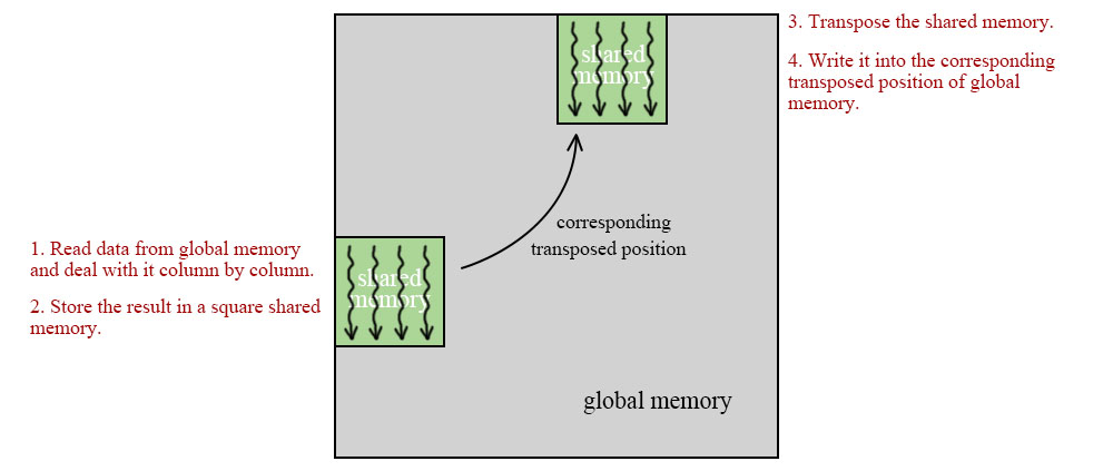
Figure 1. Transpose operation
For the 2D version of PBA source codes, Phase 2 computes the proximate sites $\mathcal{P}_i$ for each column $i$ from the 1D EDT of each row. The input to Phase 2 is $\mathcal{S}_i$ - the collection of the closest site of each pixel, and we need to remove the sites which will be dominated by the adjacent 2 sites to obtain $\mathcal{P}_i$. Assume that, in a closest site collection $\mathcal{S}_i$ $(i=x_0)$, there are 3 adjacent sites $a(x_1,y_1)$, $b(x_2,y_2)$ and $c(x_3,y_3)$, $y_1 < y_2 < y_3$, we can say that $b$ is dominated by $a$ and $c$ if $$\frac{y_1+y_2}{2}+\frac{x_2-x_1}{y_2-y_1} \cdot (\frac{x_1+x_2}{2}-x_0) > \frac{y_2+y_3}{2}+\frac{x_3-x_2}{y_3-y_2} \cdot (\frac{x_2+x_3}{2}-x_0).$$ This inequality will be computed many times, and the floating point arithmetic will take a lot of time, so we can turn it into the following form: $$[(y_2-y_1)\cdot (y_1+y_2) + (x_2-x_1)\cdot (x_1+x_2-2x_0)]\cdot (y_3-y_2) > [(y_3-y_2)\cdot (y_2+y_3) + (x_3-x_2)\cdot (x_2+x_3-2x_0)]\cdot (y_2-y_1).$$ It’s easy to understand that it will be faster and more precise than before because all the operations are now integer arithmetic.
Let’s recall how we did Phase 3 in the old approach of 2D version of PBA: we used a block coloring method that uses the set $\mathcal{P}_i$, whose sites are linked as a list in increasing $y$-coordinate, of each column $i$ to compute the closest site for each pixel $(i,\space j)$ in the order of $j=0,\space 1,...,\space n-1$. At each pixel $p$, we check the distance of $p$ to the two sites $a$ and $b$ where $b$ is the next element of $a$ in $\mathcal{P}_i$. If $a$ is closer, then $a$ is the closest site to $p$; otherwise we remove $a$ and use $b$ in place of $a$ to repeat this operation until we find the closest site of $p$. For each image column, we use $m_3$ threads to color $m_3$ consecutive pixels at a time. Each thread find the closest site of the corresponding pixel and wait for the last thread ($thread_{m_3-1}$). We synchronize the whole block and $thread_{m_3-1}$ write its answer to shared memory, then each thread deal with the next pixel and start from the last site $thread_{m_3-1}$ wrote; see Figure 2, where the same color pixels in an image column are handled by the same thread.

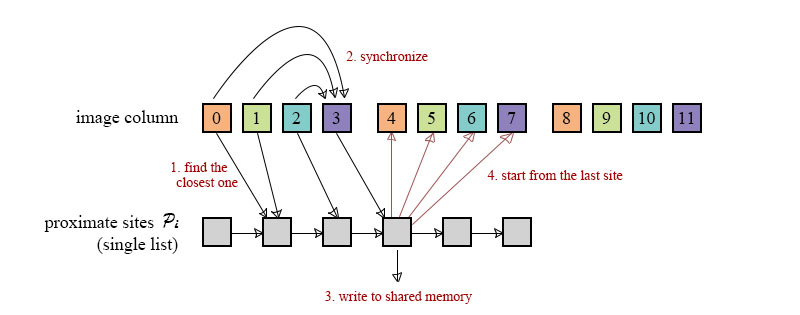
Figure 2. The block coloring method

The block coloring method can save time because some threads don't need to travel all the sites in $\mathcal{P}_i$ one by one; that is, they can skip some sites. Our new method assigns the task to each thread equally. For example, $thread_0$ deal with the pixels $(i,\space k\cdot m_3)$, $k=0,1,...,\frac{n}{m_3}-1$. Each thread completes the work independently, instead of waiting for the last thread. Each time when a thread has found the closest site $s$ of the current pixel, it jumps to the next pixel and starts from the same site $s$; see Figure 3.

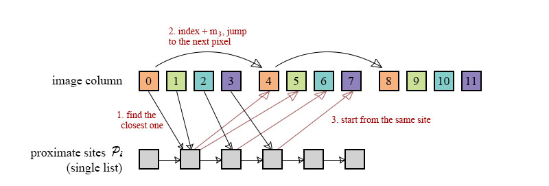
Figure 3. The new method of Phase 3

Though this new method cannot skip sites, experiments have showed that it's faster than the block coloring method. The reason is that the synchronizations in the block coloring method cost a lot of time as many threads do nothing when the threads are waiting for the last thread to complete.
For the 3D problem, we use the same methods mentioned above for 2D to improve our program. These improvements include combining the transposes, arithmetic optimization and the new method of Phase 3. There is also something different between the 2D and 3D version, in Phase 2 of 2D version, we use double linked lists to achieve linear total work, we need to change the single lists (stacks) to double lists, merge the bands and then change the double lists back to single lists for Phase 3. Because of the huge size of 3D data, in Phase 2 of 3D version, the best value of $m_2$ is $1$. This means the idea of banding plays a small role here in improving the performance because we need $O(n^2 m_2)$ $i.e.$ $O(n^2)$ threads anyway which has enough level of parallelism. It means we deal with each column with only one thread from top to bottom, and we don't need to do the single-to-double-list and double-to-single-list transforms anymore. So, we romoved these transforms because they actually cost a lot of time.
To save memory for larger input of 3D data, we compress the 3D coordinates into a single 32-bit integer $I$. See Figure 4, $I_{[29..20]}$ stores the $x$ coordinate, $I_{[19..10]}$ stores the $y$ coordinate and $I_{[9..0]}$ stores the $z$ coordinate, the remaining two bits are the flag bits. If you use the 3D version of PBA⁺, you can use the function ENCODE(x, y, z, 0, 0) (as in our source codes) to encode the coordinate of a site $(x,\space y,\space z)$ or use ENCODE(0, 0, 0, 1, 0) for non-sites, and use DECODE(pixel, x, y, z) to get the coordinate of a pixel compressed into an integer.

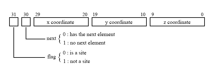
Figure 4. 3D coordinate

We have also tried the following straightforward approach to improve Phase 2. It is, however, not effective and thus not included in our PBA⁺. Here is the sketch of the attempt: for each site in $\mathcal{S}_i$ , we mark it as $0$ if it is dominated by the adjacent sites; otherwise mark it as $1$. Then we compact the array to remove all $0$s, and repeat this operation until there is no site to be removed. This method is easy but in some cases the complexity can be very bad. For the example as shown in Figure 5, there are $n$ sites (shown as blue points) on the circle, and no one can be dominated by their adjacent two sites. If there is a red site in the circle, it can dominate all the sites on the circle, but there is only one site to remove in each iteration of the above method. It means we need to repeat $O(n)$ times to get the right answer, each iteration costs $O(log\space n)$ time to compact and the total time can be $O(n\space log\space n)$.

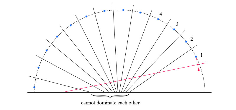
Figure 5. A bad case for the compact method

New Experiments on PBA and PBA⁺

First, we did some experiments to determine the optimal values of $m_1$, $m_2$ and $m_3$ to use in PBA⁺ on different GPUs and Table 2 shows the result. All the tests below use the appropriate values for these parameters in PBA and PBA⁺. Because of the limit of global memory, nVidia GTX 1070 and GTX 980Ti cannot deal with size of $32768^2$ and $1024^3$.

Table 2. Appropriate parameters of PBA⁺ on different GPUs

Texture Size	GTX 1070			GTX 980Ti			GTX 1080Ti
Texture Size	$m_1$	$m_2$	$m_3$	$m_1$	$m_2$	$m_3$	$m_1$	$m_2$	$m_3$
$512^2$	8	16	8	8	16	16	8	32	16
$1024^2$	16	32	8	16	16	8	16	32	16
$2048^2$	32	32	8	32	16	8	32	32	8
$4096^2$	64	32	4	64	16	4	64	32	8
$8192^2$	64	32	4	64	32	4	128	32	4
$16384^2$	128	32	4	128	32	4	128	32	4
$32768^2$	-	-	-	-	-	-	128	32	4
$64^3$	1	1	2	1	1	2	1	1	4
$128^3$	1	1	2	1	1	2	1	1	2
$256^3$	1	1	2	1	1	2	1	1	2
$512^3$	1	1	2	1	1	2	1	1	2
$768^3$	1	1	2	1	1	1	1	1	2
$1024^3$	-	-	-	-	-	-	1	1	2

Then, we did some experiments to compare PBA and PBA⁺. As PBA⁺ uses global memory only and uses some simple methods to save memory, PBA⁺ can deal with larger inputs than PBA. More specifically, on GPUs with 11GB RAM, PBA⁺ can deal with textures of size of $32768^2$ or $1024^3$ while PBA can only deal with $11264^2$ and $512^3$. We ran the test for both PBA and PBA⁺ with different inputs on nVidia GTX 1080Ti with 11GB RAM and Table 3 shows the result.

Table 3. Running time (milliseconds) of different versions with different inputs

Input	Version	$512^2$	$1024^2$	$2048^2$	$4096^2$	$8192^2$	$16384^2$	$32768^2$
0.01% random	PBA	0.19	0.35	1.02	3.97	16.71	-	-
0.01% random	PBA⁺	0.20	0.32	0.88	2.93	11.91	61.05	314.90
1% random	PBA	0.27	0.46	1.33	4.68	18.97	-	-
1% random	PBA⁺	0.25	0.45	1.26	3.99	14.54	58.75	237.04
10% random	PBA	0.32	0.57	1.68	5.79	22.74	-	-
10% random	PBA⁺	0.31	0.59	1.66	4.90	17.41	71.53	291.86
30% random	PBA	0.33	0.62	1.82	6.09	23.01	-	-
30% random	PBA⁺	0.34	0.64	1.90	5.17	17.59	71.81	281.79
50% random	PBA	0.34	0.64	1.85	6.06	22.60	-	-
50% random	PBA⁺	0.34	0.67	1.89	5.13	17.07	69.78	273.04
70% random	PBA	0.34	0.64	1.86	6.02	22.31	-	-
70% random	PBA⁺	0.31	0.65	1.82	4.87	16.11	65.96	257.04
90% random	PBA	0.31	0.66	1.99	5.96	21.84	-	-
90% random	PBA⁺	0.30	0.63	1.91	4.69	15.41	60.79	247.59

Input	Version	$64^3$	$128^3$	$256^3$	$512^3$	$768^3$	$1024^3$
0.01% random	PBA	0.31	0.74	5.68	45.17	-	-
0.01% random	PBA⁺	0.18	0.54	3.25	25.97	95.69	239.11
1% random	PBA	0.52	1.28	11.13	79.66	-	-
1% random	PBA⁺	0.29	0.78	7.16	51.39	187.87	421.83
10% random	PBA	0.60	1.33	9.40	68.25	-	-
10% random	PBA⁺	0.30	0.76	4.76	34.11	115.47	263.70
30% random	PBA	0.53	1.33	9.15	66.07	-	-
30% random	PBA⁺	0.29	0.72	4.45	31.77	106.88	242.95
50% random	PBA	0.50	1.26	8.95	64.60	-	-
50% random	PBA⁺	0.27	0.70	4.21	30.33	101.59	235.21
70% random	PBA	0.48	1.21	8.76	63.31	-	-
70% random	PBA⁺	0.25	0.66	4.09	29.08	97.58	230.75
90% random	PBA	0.43	1.14	8.12	59.55	-	-
90% random	PBA⁺	0.21	0.61	4.02	28.41	95.66	227.90

The result alludes to the fact that PBA⁺ is faster than PBA in most cases (differences of $10^{-2}$ milliseconds can be ignored) and is suitable for larger inputs. We ran the data of density of $50\%$ on different GPUs such as nVidia GTX 1070 and GTX 980Ti. Figure 6 shows the result.

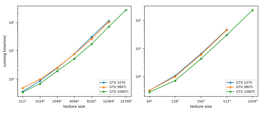
Figure 6. Running time on different GPUs

From the technical specifications of these GPUs, we see that PBA⁺ scales very well with the increase in the number of processors. To better analyse the running time of PBA⁺, we ran the data of texture size of $8192^2$ with different densities of sites and Figure 7 shows the result.

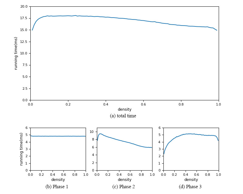
Figure 7. Running of different part with different densities

The result shows that PBA⁺ is slightly faster when there are very few sites, slower when the density is about $10\%$, and gets faster when the density increases. The reason is that the running time of Phase 1 will not be affected by the density, Phase 2 is slower when the density is about $10\%$ because there are more sites need to be removed, and less sites can be removed when the density increases, and while the sites in $\mathcal{P}_i$ are getting more and more, the running time of Phase 3 also increases.

In general, PBA⁺ utilizes the GPU better because of its high level of parallelism and good memory access pattern, and it's more efficient and can deal with larger inputs than PBA and almost all known EDT computation on the GPU.

New Version of Software: PBA⁺ Github Repositories

Dated: 28 Aug 2019

Texture Size	GTX 1070			GTX 980Ti			GTX 1080Ti
Texture Size	\(m_1\)	\(m_2\)	\(m_3\)	\(m_1\)	\(m_2\)	\(m_3\)	\(m_1\)	\(m_2\)	\(m_3\)
\(512^2\)	16	16	8	16	16	16	16	32	16
\(1024^2\)	16	32	8	16	16	8	16	32	16
\(2048^2\)	16	32	8	16	16	8	32	32	16
\(4096^2\)	32	32	4	32	16	4	64	32	8
\(8192^2\)	32	32	4	32	32	4	128	32	4
\(64^3\)	1	1	2	1	1	2	1	1	4
\(128^3\)	1	1	2	1	1	2	1	1	2
\(256^3\)	1	1	2	1	1	2	1	1	2
\(512^3\)	1	1	2	1	1	2	1	1	2