| Exploring Essential Attributes For Detecting MicroRNA Precursors From Background Sequences | |||||||||||||||||||||||||||||||||||||||||||||||||||||||||||||||||||||||||||||||||||||||||||||||||||||||||||||||||||||||||||||||||||||||||||
| Yun Zheng, Wynne Hsu, Mong Li Lee and Limsoon Wong | |||||||||||||||||||||||||||||||||||||||||||||||||||||||||||||||||||||||||||||||||||||||||||||||||||||||||||||||||||||||||||||||||||||||||||
|
Department of Computer Science School of Computing National University of Singapore Singapore 117543 Email: {zhengy, whsu, leeml, wongls}@comp.nus.edu.sg |
|||||||||||||||||||||||||||||||||||||||||||||||||||||||||||||||||||||||||||||||||||||||||||||||||||||||||||||||||||||||||||||||||||||||||||
| Abstract | |||||||||||||||||||||||||||||||||||||||||||||||||||||||||||||||||||||||||||||||||||||||||||||||||||||||||||||||||||||||||||||||||||||||||||
| MicroRNAs (miRNAs) have been shown to play important roles in different biological processes, especially in post-transcriptional gene regulation. The hairpin structure is a key characteristic of the microRNAs precursors (pre-miRNAs). How to encode their hairpin structures is a critical step to correctly detect the pre-miRNAs from background sequences, i.e., pseudo miRNA precursors. In this paper, we have proposed to encode the hairpin structures of the pre-miRNA with a set of features, which captures both the global and local structure characteristics of the pre-miRNAs. Furthermore, we find that four essential attributes, with both global and local features, are discriminatory for classifying human pre-miRNAs and background sequences. The experimental results show that the number of conserved essential features decreases when the phylogenetic distance between the species increases. Specifically, one A-U pair, which produces the U at the start position of most mature miRNAs, in the pre-miRNAs is found to be well conserved in different species for the purpose of biogenesis. | |||||||||||||||||||||||||||||||||||||||||||||||||||||||||||||||||||||||||||||||||||||||||||||||||||||||||||||||||||||||||||||||||||||||||||
|
NOTE: |
|||||||||||||||||||||||||||||||||||||||||||||||||||||||||||||||||||||||||||||||||||||||||||||||||||||||||||||||||||||||||||||||||||||||||||
The DFLearner software provided here is free for academic purpose. Please cite the following papers when using the DFLearner software in scientific publications. Zheng Yun and Kwoh Chee Keong. Dynamic Algorithm for Inferring Qualitative Models of Gene Regulatory Networks. Proceedings of the 3rd Computer Society Bioinformatics conference, CSB 2004.pages: 353-364. IEEE Computer Society Press. 2004 [pdf] [slides] Zheng Yun and Kwoh Chee Keong. Identifying simple discriminatory gene vectors with an information theory approach. In Proceedings of the 4th Computational Systems Bioinformatics Conference, CSB 2005, pages:12-23. IEEE Computer Society Press, 2005. [pdf] [slides] [supplements] |
|||||||||||||||||||||||||||||||||||||||||||||||||||||||||||||||||||||||||||||||||||||||||||||||||||||||||||||||||||||||||||||||||||||||||||
| Supplements | |||||||||||||||||||||||||||||||||||||||||||||||||||||||||||||||||||||||||||||||||||||||||||||||||||||||||||||||||||||||||||||||||||||||||||
| The Discrete
Function Learner (DFLearner) software (1.2MB)
Include the software and the data files for some examples in the paper. Current version has been validated on Windows and HP Tru64 Unix platform. |
software.zip | ||||||||||||||||||||||||||||||||||||||||||||||||||||||||||||||||||||||||||||||||||||||||||||||||||||||||||||||||||||||||||||||||||||||||||
| The miREncoding
software
This software inputs the pre-miRNA sequences together with the secondary structure of them, then encode the sequences into 43 features. |
miREncoding.zip | ||||||||||||||||||||||||||||||||||||||||||||||||||||||||||||||||||||||||||||||||||||||||||||||||||||||||||||||||||||||||||||||||||||||||||
| Data sets | data.zip | ||||||||||||||||||||||||||||||||||||||||||||||||||||||||||||||||||||||||||||||||||||||||||||||||||||||||||||||||||||||||||||||||||||||||||
| A Brief Introduction to the Discrete Function Learning algorithm | Chapter 1 of Online Help of the DFLeaner | ||||||||||||||||||||||||||||||||||||||||||||||||||||||||||||||||||||||||||||||||||||||||||||||||||||||||||||||||||||||||||||||||||||||||||
| The Weka software
In our experiments, we use the GUI version 3.4.2. |
http://www.cs.waikato.ac.nz/~ml/weka/ | ||||||||||||||||||||||||||||||||||||||||||||||||||||||||||||||||||||||||||||||||||||||||||||||||||||||||||||||||||||||||||||||||||||||||||
| Original data
sets
We use pre-miRNAs in the release 5.0 of the miRBase Sequence Database. |
|||||||||||||||||||||||||||||||||||||||||||||||||||||||||||||||||||||||||||||||||||||||||||||||||||||||||||||||||||||||||||||||||||||||||||
| Selection of Parameters of the Discrete Function Learning algorithm | Supplementary Section S1. | ||||||||||||||||||||||||||||||||||||||||||||||||||||||||||||||||||||||||||||||||||||||||||||||||||||||||||||||||||||||||||||||||||||||||||
| Supplementary Figures | |||||||||||||||||||||||||||||||||||||||||||||||||||||||||||||||||||||||||||||||||||||||||||||||||||||||||||||||||||||||||||||||||||||||||||
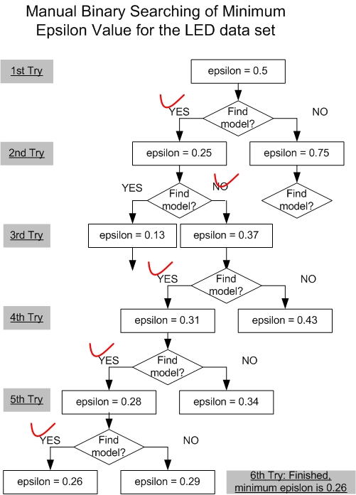
| The manual binary search of minimum ε value. | Figure S1. | ||||||||||||||||||||||||||||||||||||||||||||||||||||||||||||||||||||||||||||||||||||||||||||||||||||||||||||||||||||||||||||||||||||||||||
| The selection of essential attributes with the DFL algorithm. | Figure S2. | ||||||||||||||||||||||||||||||||||||||||||||||||||||||||||||||||||||||||||||||||||||||||||||||||||||||||||||||||||||||||||||||||||||||||||
| Supplementary Tables | |||||||||||||||||||||||||||||||||||||||||||||||||||||||||||||||||||||||||||||||||||||||||||||||||||||||||||||||||||||||||||||||||||||||||||
| The summary of data sets. | Table S1. | ||||||||||||||||||||||||||||||||||||||||||||||||||||||||||||||||||||||||||||||||||||||||||||||||||||||||||||||||||||||||||||||||||||||||||
| The prediction accuracies of different classification algorithms on the data sets with all features. | Table S2. | ||||||||||||||||||||||||||||||||||||||||||||||||||||||||||||||||||||||||||||||||||||||||||||||||||||||||||||||||||||||||||||||||||||||||||
| The prediction accuracies of different classification algorithms on the data sets with 32 local features. | Table S3. | ||||||||||||||||||||||||||||||||||||||||||||||||||||||||||||||||||||||||||||||||||||||||||||||||||||||||||||||||||||||||||||||||||||||||||
| The prediction accuracies of different classification algorithms on the data sets with 11 global features. | Table S4. | ||||||||||||||||||||||||||||||||||||||||||||||||||||||||||||||||||||||||||||||||||||||||||||||||||||||||||||||||||||||||||||||||||||||||||
| The prediction accuracies of different classification algorithms on the data sets with the features chosen by the DFL algorithm. | Table S5. | ||||||||||||||||||||||||||||||||||||||||||||||||||||||||||||||||||||||||||||||||||||||||||||||||||||||||||||||||||||||||||||||||||||||||||
| Supplementary Section S1: Selection of Parameters | |||||||||||||||||||||||||||||||||||||||||||||||||||||||||||||||||||||||||||||||||||||||||||||||||||||||||||||||||||||||||||||||||||||||||||
| We discuss how to select the two parameters, the expected cardinality of the EAs K and the ε value, of the Discrete Function Learning algorithm in this section. | |||||||||||||||||||||||||||||||||||||||||||||||||||||||||||||||||||||||||||||||||||||||||||||||||||||||||||||||||||||||||||||||||||||||||||
|
S1.1 The Selection of The Expected Cardinality K We discuss the selection of K in this section. Generally, if a
data set has a large number of features, like several thousands, then K can be assigned to a small constant, like 50, since the
models with large number of features will be very difficult to understand. If the number of features is small, then the
K can be directly specified to the number of features n. S1.2 The Selection of The ε Value For a given noisy data set, the missing part of
H(Y), as demonstrated in Figure 1.4, is determined, i.e., there exists a specific minimum ε
value, ε_m, with which the DFL algorithm can find the original
model. If the ε value is smaller than the ε_m, the DFL algorithm will not find the original
model. Here, we will
introduce two methods to efficiently find the ε_m. We use the LED data sets with 10 percent noise to shown the procedure. For this example, in the first try, DFL algorithm finds a model with ε of 0.5. Then, the DFL algorithm cannot find a model with the ε of 0.25 in the second try. Similarly, in the 3rd to 6th tries, the DFL algorithm finds models with the specified ε values, 0.37, 0.31, 0.28 and 0.26. Since we have known in the second try that the DFL algorithm cannot find a model with ε of 0.25. Hence, 0.26 is the minimum ε value for this data set. Figure S1. The manual binary search of minimum ε value.
|
|||||||||||||||||||||||||||||||||||||||||||||||||||||||||||||||||||||||||||||||||||||||||||||||||||||||||||||||||||||||||||||||||||||||||||
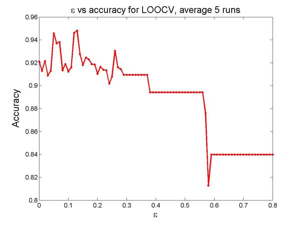
| Figure
S2. The selection of essential attributes with the DFL algorithm.
To find the best subset of EAs for the data sets, we first set the expected cardinality of the EAs K as 10. Next, we use the DFL algorithm to perform leave-one-out cross validation (LOOCV) on the training set (TR-C) with different ε values, from 0 to 0.8 with a step of 0.01. Then, we find that the DFL algorithm reaches its best prediction performance in the LOOCV when ε within [0.12, 0.13]. When using all samples in training data set, the distributions of attributes are slightly different from those in LOOCV. Thus, we try the DFL classifiers obtained from a wider region of ε within [0.1, 0.15]. Finally, we choose the DFL classifier obtained when ε = 0.11 because it shows overall better prediction accuracies for data set 1 to 4. In this way, a subset of 4 features, {A(((, G·((, length basepair ratio, energy per nucleotide}, is chosen as EAs for the human data sets, D1 to D4. For other data sets, we try the subsets of these 4 EAs and choose those subsets on which the 1NN algorithm introduced in Section 3.5 produces the best prediction performances. The selected EAs are shown in Figure 3 (a).As shown in Figure S2, there is another region of ε around 0.5 within which the DFL algorithm achieves high prediction accuracy in cross validation. But the DFL models use more features when ε decreases. Thus, we prefer the features chosen by the DFL algorithm when ε is in the region of [0.1,0.15].
|
|||||||||||||||||||||||||||||||||||||||||||||||||||||||||||||||||||||||||||||||||||||||||||||||||||||||||||||||||||||||||||||||||||||||||||
Table
S1. The summary of data sets.
In this research, we use the data sets in
literature (Xue et al. 2005) to validate our approach, since it is
valuable to compare the published results. These data sets are
summarized in Table S1. Data set 0 to 4 is from human, and data set 5 to
15 is from other species, as indicated by their names. Data set 0 is
used as the training data set, and data set 1 to 15 are used as testing
data sets. There are totally 4094 samples used as testing data sets,
with 3444 background sequences and 650 pre-miRNAs.
|
|||||||||||||||||||||||||||||||||||||||||||||||||||||||||||||||||||||||||||||||||||||||||||||||||||||||||||||||||||||||||||||||||||||||||||
Table
S2. The prediction accuracies of different classification algorithms on
the data sets with all features.
|
|||||||||||||||||||||||||||||||||||||||||||||||||||||||||||||||||||||||||||||||||||||||||||||||||||||||||||||||||||||||||||||||||||||||||||
Table
S3. The prediction accuracies of different classification algorithms on
the data sets with 32 local features.
$ For the local data sets, the prediction accuracies of the SVM algorithm in our study are slightly better than those in literature (Xue et al. 2005). We contribute this to the encoding region in our research. We encode the triplet local features for the whole pre-miRNAs, except the first and last nucleotide. However, only the paired regions of the pre-miRNAs are encoded into triplet features in (Xue et al. 2005). * The Tri-SVM column shows the results from literature (Xue et al. 2005). |
|||||||||||||||||||||||||||||||||||||||||||||||||||||||||||||||||||||||||||||||||||||||||||||||||||||||||||||||||||||||||||||||||||||||||||
Table
S4. The prediction accuracies of different classification algorithms on
the data sets with 11 global features.
|
|||||||||||||||||||||||||||||||||||||||||||||||||||||||||||||||||||||||||||||||||||||||||||||||||||||||||||||||||||||||||||||||||||||||||||
Table
S5. The prediction accuracies of different classification algorithms on
the data sets with the features chosen by the DFL algorithm.
|
|||||||||||||||||||||||||||||||||||||||||||||||||||||||||||||||||||||||||||||||||||||||||||||||||||||||||||||||||||||||||||||||||||||||||||
|
References: 1. I. Bentwich, A. Avniel, Y. Karov, R. Aharonov, S. Gilad, O. Barad, A. Barzilai, P. Einat, U. Einav, E. Meiri, E. Sharon, Y. Spector, and Z. Bentwich. Identification of hundreds of conserved and nonconserved human micrornas. Nature Genetics, 37(7):766–70, 2005. 2. S. Griffiths-Jones. The microRNA Registry. Nucl. Acids Res., 32(90001):D109–111, 2004. 3. I.L. Hofacker. Vienna RNA secondary structure server. Nucl. Acids Res., 31(13):3429–3431, 2003. 4. D. Karolchik, R. Baertsch, M. Diekhans, T.S. Furey, A. Hinrichs, Y.T. Lu, K.M. Roskin, M. Schwartz, C.W. Sugnet, D.J. Thomas, R.J. Weber, D. Haussler, and W.J. Kent. The UCSC Genome Browser Database. Nucl. Acids Res., 31(1):51–54, 2003. 5. C. Xue, F. Li, T. He, G.-P. Liu, Y. Li, and X. Zhang. Classification of real and pseudo microRNA precursors using local structure-sequence features and support vector machine. BMC Bioinformatics, 6(1):310, 2005.
|
|||||||||||||||||||||||||||||||||||||||||||||||||||||||||||||||||||||||||||||||||||||||||||||||||||||||||||||||||||||||||||||||||||||||||||