Attention Saturation
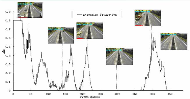
The evolution of temporal attention (attention saturation) is shown in Figure 1. Figure 1 shows that the temporal motion attention, calculated from the equation (24), evolves according to the motion activity in a traffic sequence. The NA , attention saturation, roughly reflects the traffic status at each time step. Therefore, our method here can be used for monitoring the traffic also. It also shows that the temporal attention is aroused only when the cars pass by. At other times, when NA is zero, there are no attention samples. During this time, the only processing and analysis done is the sensor sampling. It should be understood that all the results are obtained by only processing a few samples in the visual data. There is no need to process the entire data. It fulfills our aims of providing analysis have the ability to select the data to be processed.
Experiential Sampling
4. Experimental Results
Figure 1. Temperal attention via attention saturation
Computation Speed
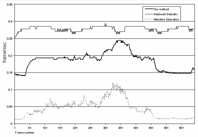
We use a USB web camera to perform real time face detection on a Pentium III 1GHz laptop. The graph of the computation load (with frame capturing, rendering, recording results (saving to disks), etc.) in this real time scenario is shown in Figure 2. Note that our absolute speed is constrained by the capture speed of the USB camera. However, we intend to show the adaptability of our computational load rather than the absolute speed. In Figure 2, curve 1 shows the computation load of the adaboost face detection while curve 2 indicates the computation load of our experiential sampling with adaboost face detector. This figure shows that by using our experiential sampling technique, computation complexity can be significantly reduced. In addition, in order to show the adaptability, we also depict the value of attention saturation in the graph. It shows that the computation complexity varies according to the difficulty of the current task, which is measured by the attention saturation.
Figure 2. Computation Speed
Past Experience
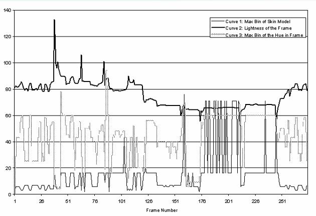
We have implemented the use of the past experience for building the dynamic skin color model. The experimental results are shown in Figure 3. We change the luminance of our visual scene. This consequently causes the global visual environment to vary, which is indicated by the curve 1 (luminance) and curve 2 (Max bin in hue) as shown in Figure 3. By constantly updating the skin color model from the previous analysis, our skin color model can dynamically adapt to the changed visual environment.
Figure 3. Adaptive skin color model via past experience
Experiential Sampling