Function Call

Learning Objectives

At the end of this sub-unit, students should

appreciate the improved readability by naming a sequence of operations.
know how to invoke functions.
know how to accept the return value from functions.
know how to chain functions.

Naming Operations

Our motivation is still captured by the quote by John Woods.

Quote

"Always code as if the guy who ends up maintaining your code will be a violent psychopath who knows where you live. Code for readability."

John Woods

Let us look back at the partial solution for \(e^x\) and \(\binom{m}{k}\).

\(e^x\)\(\binom{m}{k}\)

# input: x, k  (we use k because we cannot use n)
i = 0
e = 0  # local, will be our result
while i < k:
  n = i
  # res <- n!
  e = e + ((x ** i) / res)
  i = i + 1
print(e)

# input: m, k
# compute m!
n = m
# res <- n!
fact_m = res

# compute k!
n = k
# res <- n!
fact_k = res

# compute (m-k)!
n = m - k
# res <- n!
fact_mk = res

binom = fact_m / (fact_k * fact_mk)  # m! / (k! (m-k)!)
print(binom)

We abstracted the factorial problem and say that we can solve it as we have a code for it. Unfortunately, to use it, we have to use tricky conventions so that there is no name clashes. Wouldn't it be nice if there is a way to do this more cleanly without all of these conventions? After all, we are humans and we may make mistakes during the renaming and composition. A direct support from the Python language will be beneficial.

Luckily, we are not the first people to want this. There is indeed a support from Python called function call. With functions, we can rewrite the two code above as follows assuming that we have a function called factorial.

\(e^x\)\(\binom{m}{k}\)

# input: x, k  (we use k because we cannot use n)
i = 0
e = 0  # local, will be our result
while i < k:
  res = factorial(i)
  e = e + ((x ** i) / res)
  i = i + 1
print(e)

# input: m, k
fact_m = factorial(m)      # compute m!
fact_k = factorial(k)      # compute k!
fact_mk = factorial(m - k) # compute (m - k)!
binom = fact_m / (fact_k * fact_mk)  # m! / (k! (m-k)!)
print(binom)

Now that is a more readable code. There is another advantage here. We do not have to know how the factorial is computed. The code for that is irrelevant. It can be any of the following.

It is the code we have written before, but someone is computing it with pen and paper.
The number n is emailed to a student and the student spent their free time computing the factorial of n and email us back the answer.
Someone has drawn the graph for \(\Gamma(x)\) function and they simply draw a straight line from \(x + 1\) and look at the corresponding value on the \(y\)-coordinate.

The main thing is, if we are simply using the function, we do not care how the function is written. We only need to know the function specification and how to use the function. This is called function invocation.

Invoking Functions

We have done this before, but we have a very limited of functions to show the actual behavior and potential complications. So let us introduce more functions from the mathematic library in the math module.

Function	Description
`factorial(n)`	Returns the factorial of the integer `n`
`comb(n, k)`	Returns the value of \(\binom{n}{k}\)

You may have noticed that the functions introduced above are exactly what we have written before. It would have been easier if we have used them. But it is a good exercise to be able to implement them as you may not always use a language that have those functions implemented. To actually use these functions, you will need to add the following import declaration at the beginning of your code.

from math import *

So let us assume we have them. This additional step should not distract us from what we need to learn here and that is, how do we use these functions.

First, notice the way we specify the function. In factorial, we specify the name n within parentheses. This corresponds to the way we represent our own factorial as a grey box, shown below.

Grey05

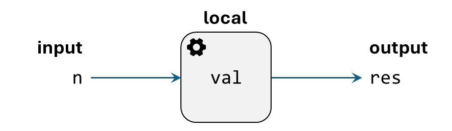
The input n is exactly the n inside the parentheses of factorial(n). But now we do not care about the implementation of factorial. So we do not care about local variables. This is good, because we may accidentally use the same variable name but it will not interfere with the working of this function.

Secondly, we do not care what is the variable that stores the resulting output. Because clearly that has been defined locally and we say that we do not care about the internals. So we will instead say that there is going to be a value produced and we will describe what this value is. This actually corresponds to the description of the function in the table. We use the terminology returns here because as you will see later, it will correspond to the keyword we will use.

But the main idea is that we can now change the grey box into a black box. One that we do not care about the internals.

Black01

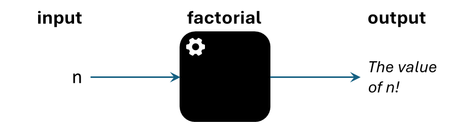
The same specification factorial(n) also describes the way we can invoke the function. We simply use the name, add parentheses after the name, and provide values within the parentheses. Three things to note about these values.

The value need not be a constant value (e.g., 3), but it can be a variable and/or expressions that is evaluated into a value.
The number of values must match the number of inputs that the function accepts.
We call these values as arguments.

Function Invocation of Factorial

Correct function invocation with correct number of values.

>>> from math import *
>>> factorial(10)    # the argument can be values
3628800
>>> x = 5
>>> factorial(x)     # the argument can be variables
120
>>> factorial(x + x) # the argument can be expression
3628800

Incorrect function invocation with incorrect number of values.

>>> factorial()      # 0 arguments
TypeError
>>> factorial(1, 2)  # 2 arguments
TypeError

It has been a while since we use the IDLE REPL so let us remind you that we see something printed because there is a value produced by the function. This printing is because of P in REPL. If we run the code from the editor, we will not see anything printed. To remember the value produced, we should assign it to a variable. In fact, this is what we did above. The code is reproduced below with the addition of the import statement.

\(e^x\)\(\binom{m}{k}\)

from math import *
# input: x, k  (we use k because we cannot use n)
i = 0
e = 0  # local, will be our result
while i < k:
  res = factorial(i)   # assigned to res
  e = e + ((x ** i) / res)
  i = i + 1
print(e)

from math import *
# input: m, k
fact_m = factorial(m)      # compute m!
fact_k = factorial(k)      # compute k!
fact_mk = factorial(m - k) # compute (m - k)!
binom = fact_m / (fact_k * fact_mk)  # m! / (k! (m-k)!)
print(binom)

What We Did Before

We did something similar to this "passing of values". But we did it more explicitly. We started this in the left triangle problem. In that code, we prepared the argument using the following part of the code.

k = i + 1  # row construction input is k
# row construction
# ----------------------------------------
# input: k
m = k

Here, m is the counterpart of n in factorial(n) and k is the argument.

Multiple Inputs

In the case of factorial, we only have one input. So there is no ambiguity to which variables accept which inputs because there is only one possibility. But what if we have multiple inputs like comb(n, k)? Let us look at the black box representation of it first.

Black02

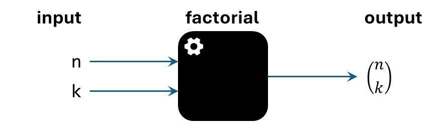
Unfortunately, we cannot really look at what we did before because the order does not matter. We used a different convention which is based on name as shown below for right triangle problem.

What We Did Before

We did something similar to this "passing of values". But we did it more explicitly. We started this in the right triangle problem. In that code, we prepared the argument using the following part of the code.

k = i + 1  # row construction input is k
# row construction
# ----------------------------------------
# input: k, n
m1 = k
m2 = n

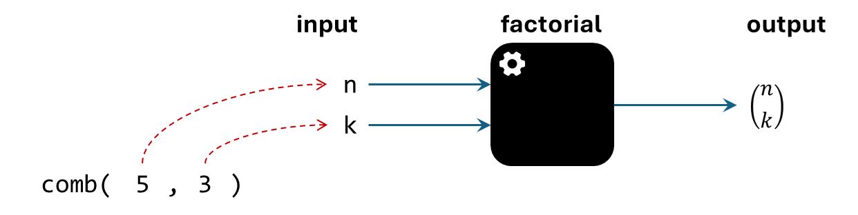
So what is the convention for function call? The simplest convention is that we use position instead of name. Before we explain the mechanism, we will first give a name to the variable that will accept the argument. We will call this parameters¹.

Evaluate the 1^st argument into a value \(V_1\) and assign \(V_1\) to the 1^st parameter.
Evaluate the 2^nd argument into a value \(V_2\) and assign \(V_2\) to the 2^nd parameter.
Evaluate the 3^rd argument into a value \(V_3\) and assign \(V_3\) to the 3^rd parameter.
and so on

As we have seen, if the number of arguments is different from the number of parameters, then we get TypeError. This mechanism of passing argument to parameter is called parameter passing. There are different conventions for these and the convention used by Python is called call by value.

Function Invocation of Combination

Correct function invocation with correct number of values.

>>> from math import *
>>> comb(5, 3)
10
>>> x = 5
>>> comb(x, 3)
10
>>> comb(x + x, x)
252

Incorrect function invocation with incorrect number of values.

>>> comb()         # 0 arguments
TypeError
>>> comb(1)        # 1 argument
TypeError
>>> comb(1, 2, 3)  # 3 arguments
TypeError

We can visualize call by value for comb(5, 3) as follows.

CBV01

No Argument?

Currently we do not have an example of functions that does not take any arguments. But it is possible to have functions that do not take in any arguments. Something we have learnt and close to having no argument is the print function because we can actually invoke it without any argument as follows.

>>> print()

>>> # an empty line is printed above

However, print is actually a much more complicated function that that because it can be called with any number of arguments. This is what we call variadic function and it is beyond the scope of our current discussion. What you should note is simply that even if there is no argument expected, we still need to put parentheses after the function name.

??? danger "Bad Practice" Due to the complexity of Python, there will be no error if we actually forgot the parentheses. But the reason is because of higher-order function. You will see the following if you forgot the parentheses.

```pycon
>>> print
<built-in function print>
```

Chaining

If we look at the way we can accept the return value of factorial(n) closely, we will realize an interesting fact. Function call is treated as an expression because in lhs = rhs, we allow rhs to be any expression. So now, in any places that accept expression, we can use function call. This means that if we want to get a value that is one more than the factorial of \(n\), we can simply write it as follows.

from math import *
one_more_than_fact_n = 1 + factorial(n)
print(one_more_than_fact_n)

Logically, if we are given \(n\), and we want to find \((n! + 1)!\)², then we can write it as a sequence of statements like the following code. We will also exclude from math import * from our notes from this point onwards and assume that all the necessary modules are imported. Also, we will exclude print to prepare ourselves for solving problems with functions.

# Assume n is initialized
fact_n_plus_1 = factorial(n) + 1
res = factorial(fact_n_plus_1)

But this is exactly the same as if we are not using the variable fact_n_plus_1 and instead, copying the rhs directly inside. This is the reverse of our way of making the code more readable. We are doing this because it reveals interesting property about functions, we can chain them.

# Assume n is initialized
res = factorial(factorial(n) + 1)

Chaining function calls allows us to write shorter code. But it may be less readable. So while this technique is interesting, use it with care. The main aspect we want to highlight is the order of operation.

Since the last two codes above are equivalent, it means that the order of operation should be the same too. This implies that the argument of a function call will be evaluated before the function call. This is captured by the motto of the expression evaluation.

Leftmost Innermost.

Let us illustrate the motto by evaluating x + factorial(factorial(y + 2) + 3). We will be highlight the sub-expressions to be evaluated and add comments for clarity. Our current state will be the following.

{ x ↦ 2 , y ↦ 3 }

x + factorial(factorial(y + 2) + 3)
  ⇒ x + factorial(factorial(y + 2) + 3)   [leftmost]
  ⇒ 2 + factorial(factorial(y + 2) + 3)   [substitute]
  ⇒ 2 + factorial(factorial(y + 2) + 3)   [leftmost]
  ⇒ 2 + factorial(factorial(y + 2) + 3)   [innermost]
  ⇒ 2 + factorial(factorial(y + 2) + 3)   [leftmost]
  ⇒ 2 + factorial(factorial(y + 2) + 3)   [innermost]
  ⇒ 2 + factorial(factorial(y + 2) + 3)   [leftmost]
  ⇒ 2 + factorial(factorial(3 + 2) + 3)   [substitute]
  ⇒ 2 + factorial(factorial(3 + 2) + 3)   [innermost]
  ⇒ 2 + factorial(factorial(5) + 3)       [evaluate]
  ⇒ 2 + factorial(factorial(5) + 3)       [leftmost-innermost]
  ⇒ 2 + factorial(120 + 3)                [evaluate]
  ⇒ 2 + factorial(120 + 3)                [leftmost-innermost]
  ⇒ 2 + factorial(123)                    [evaluate]
  ⇒ 2 + factorial(123)                    [leftmost-innermost]

At this point, the value is so large that it does not make sense to write them down. But hopefully you get the point. We evaluate the leftmost innermost sub-expressions that are not yet evaluated. In other words, if it is not yet a value, we evaluate them to produce a value.

Try to do the evaluation slowly first. Once you have gained enough practice, you should be able to reasonably evaluate any function call. Let us show some quick evaluation using another example by highlighting only the next evaluated expression directly.

{ x ↦ 2 , y ↦ 3 }

comb(factorial(y), factorial(x))
  ⇒ comb(factorial(y), factorial(x))
  ⇒ comb(factorial(3), factorial(x))
  ⇒ comb(6, factorial(x))
  ⇒ comb(6, factorial(2))
  ⇒ comb(6, 2)
  ⇒ 15

Nothing

There are functions that do not return anything. Put it another way, it returns nothing. But what is nothing? This is philosophical conundrum because as soon as we identify what "nothing" is, it becomes something. Luckily, we are not philosophers, we are computer scientist. So we can simply say that we have a value to represent nothing. This type is called the NoneType and there is only one value of this type called None.

Adapted to Python

"None means "Boring". It means the boring type which contains one thing, also boring. There is nothing interesting to be gained by comparing one element of the boring type with another, because there is nothing to learn about an element of the boring type by giving it any of your attention.

It is very different from the empty type [...]. The empty type is very exciting, because if somebody ever gives you a value belonging to it, you know that you are already dead and in Heaven and that anything you want is yours."

Conor McBride

So while we cannot represent true nothingness (i.e., empty), we can represent something quite close to it. Since there is only one value in NoneType, which is None, we will use these two interchangeably. The usage of None in Python is actually far from boring. Because it represents nothing, if a function returns nothing, it actually returns None.

IDLE REPL also behave differently in the presence of None. In particular, because it represents nothing, the P in REPL prints nothing when presented by the value None. This is really nothing because nothing is printed.

>>> None
>>> # no print!

That is not a typo. We can even try assigning None to a variable and try to get the value in IDLE. It will still print nothing.

>>> x = None
>>> x
>>> # still no print!

If we really want to print None, we need to use print(None).

>>> print(None)
None

You are probably wondering, but what is the return value of the print function? The code above actually already has the answer. Let us reason about this slowly before proving that our reasoning is indeed correct.

First, we know that None is not printed by IDLE unless we use print(None). Second, we know that function returns something. From here, we can deduce that print is returning something that is not printed by IDLE. The None above is printed by the function, not from the return value of print. Therefore, we can conclude that print must return None. In other words, it returns nothing.

So that is our reasoning. How do we know we are correct? That is easy, we can assign the return value of print to a variable and check what is that value.

>>> is_none = print(2)  # the 2 below is printed by the print function, not IDLE
2
>>> is_none
>>> print(is_none)      # we will see None if is_none has the value None
None

Now test your understanding, what will be printed by the following code?

CodeAnswer

print(print(None))

None
None

Others may use parameters and arguments interchangeably. Another alternative is to call arguments as actual parameters and parameters as formal parameters. We choose to differentiate them for simplicity. ↩
That is, performing factorial twice. ↩