MIPS Language
Objective
At the end of this chapter, you should be able to:
- Read MIPS programs.
- Write MIPS programs.
- Trace MIPS programs.
- Compile C to MIPS.
- Assemble MIPS to machine code (i.e., binary).
Recap
We now have the basic knowledge needed to start our exploration of the MIPS assembly language. First, recap the overall process of compilation.
You write programs in high-level programming languages such as C/C++, Java, etc:
| Add | |
|---|---|
1 | |
Compiler translates this into assembly language statement:
| Add | |
|---|---|
1 | |
Assembler translates this statement into machine language instructions:
| Add | |
|---|---|
1 | |
Note that processors can only execute binary instructions. While we often write this as numbers 0 or 1, in the actual machine, it is often represented as high voltage or low voltage. One possible representation of the machine instruction above is as follows:

Note that the representation is not the only possible representation and you will learn in the second half of the module how to operate on these.
Instruction Set Architecture
Fortunately, we are not going to deal with voltages directly. Instead, we will deal with an abstraction of one. We will often abstract away the hardware into interface that we call instruction set architecture (ISA).
The ISA includes everything programmers need to know to make machine code work correctly. Additionally, ISA also allows computer designer to talk about functions independently from the hardware that performs them. Which means, at this point, we do not care about the lines (which is the signal) but only care about the abstracted value (i.e., the 0s and 1s). That will be the lowest level we will go in this module.
This abstraction allows many implementations of varying cost and performance to run identical software. For example, we have Intel x86 or IA-32 ISA that has been implemented by a range of processors. These processors include 80386 from Intel produced in 1985 to Pentium 4 produced in 2005 also by Intel.
However, Intel is not the only company to have implemented these. Other companies such as AMD and Transmeta have also implemented IA-32 ISA. Which means, a program compiled for IA-32 ISA can be executed on any of these implementations.
Assembly Language vs Machine Code
Note that typically the translation from assembly language to machine code is usually one-to-one. So for most practical purposes, we treat them as equivalent. However, there are still differences between them:
| Assembly Language | Machine Code |
|---|---|
| Symbolic version of machine code | Instructions are represented in binary |
| Human readable | Technically readable, but hard and tedious for programmer |
add A, B |
1000 1100 1010 0000 |
Assembler is the tool to translate assembly language to machine code. Additionally, assembly language may provide pseudo-instructions as syntactic sugar. These syntactic sugar will then be translated into one or more real instructions. When we consider performance, we will only count the real instructions.
Walkthrough
Let us take a journey with the execution of a simple code. We have the following mini-objectives:
- Discover the components in a typical computer.
- Learn the type of instructions required to control the processor.
The illustrations here are simplified to highlight the important concepts.
Example Code
| Simple Sum | |
|---|---|
1 2 3 4 | |
| Simple Sum | |
|---|---|
1 2 3 4 | |
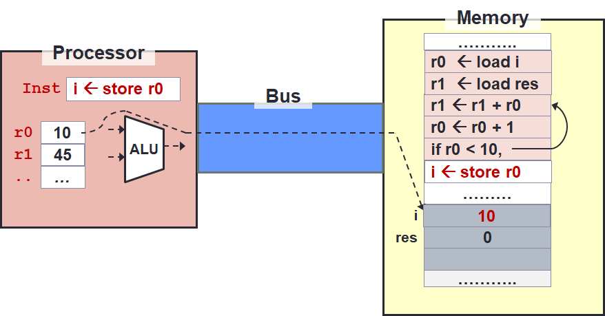
The Components
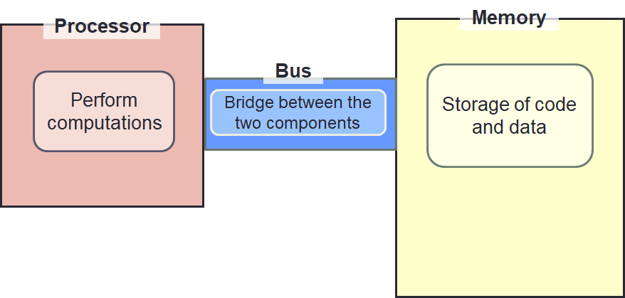
We are using the von Neumann architecture. However, we simplify this to highlight two major components:
- Processor: Perform computations.
- Memory: Storage of code and data.
We exclude input/output devices. To connect the processor and memory, we add a bus. This is simply a bridge between the two components.
The Code in Action
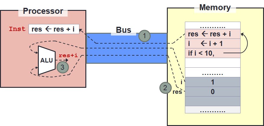
Since we are using von Neumann architecture, both the code and data reside in memory. During execution:
- The instruction from the code is transferred into the processor at the start of the execution cycle via the bus.
- During execution, the processor may request for data from memory via the bus.
- The instruction is then executed by the processor to produce the result.
- This result may then be written back to the memory.
Registers
Memory access is slow! There are many reasons for this, the simplest of which is simply the distance from the processor to the memory1. The longer the distance, the more time it takes to transfer the data.
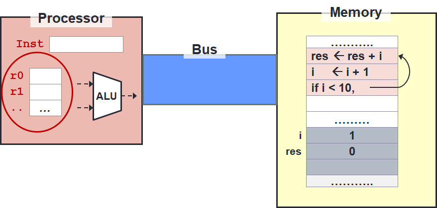
To avoid frequent access to memory, processor provides temporary storage for values near the processor called the registers.
In our toy example on the right, the registers are circled.
They are named r0, r1, etc.
The register is useful for variables that are frequently accessed.
For instance, consider the variables res and i.
Since they are in a loop, these variables will be used at least 10 times.
So it does not make sense to keep on requesting these values from memory and writing them back.
Memory Instruction
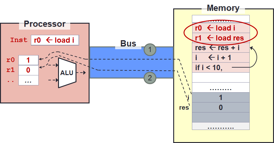
We need instruction to move data into registers.
This can be done using the load instruction (or their variants, but the main idea is the same so just memorise the concept and search for the actual keyword to be used).
We will also need to move data from registers to memory later.
This is done using the store instruction.
| Load as Mapping | |
|---|---|
1 2 | |
Register-to-Register Arithmetic
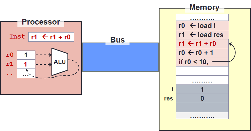
Now that the data are in registers instead of memory, we can change the operation to work directly on registers which is much faster. The changes are captured below.
| Register-to-Register Arithmetic | |
|---|---|
1 2 3 4 5 | |
Running the instruction at line 3, we see the result shown on the right above.
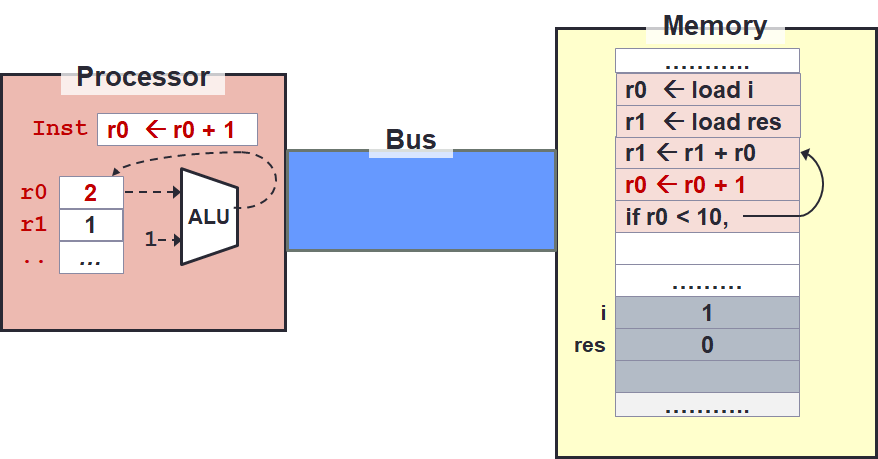
Sometimes, arithmetic operation uses a constant value instead of register value. This is exemplified by the instruction at line 4. So where does the constant come from? You will learn later that this constant is actually encoded in the instruction itself.
Execution Sequence
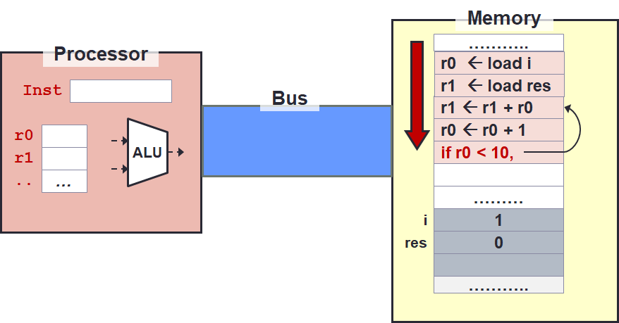
By default, instructions are executed sequentially from top to bottom. This means after the instruction at line 5, the "default" next instruction should be the instruction at the hypothetical line 6. So how do we repeat or "make a choice"?

There are several instructions to change the control flow based on condition.
The instruction we highlight here is the if (cond) goto2 instruction.
In fact, using this instruction (or its variants), both repetition (i.e., loop) and selection (i.e., if-else) can both be supported.
The idea is that repetition simply go to any line above!
The execution will then continue sequentially until we see another control flow instruction.
End of Loop
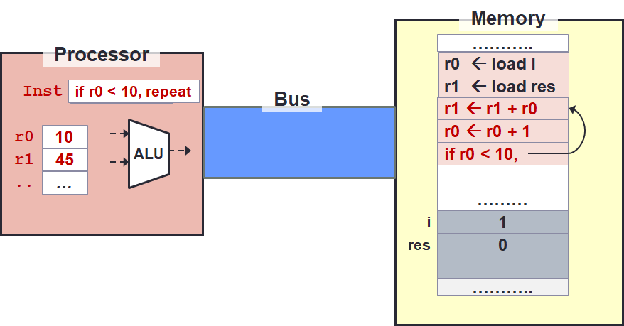
The three instructions at line 3 to line 5 will be repeated until the condition at line 5 fails. The end result will look like the image on the right.
What we want to do now is to move the value of the result back from the register to their "home" in memory.
Since we have done the mapping r0 ⇆ i and r1 ⇆ res, we can use this mapping to store the result back.
This is done using the store instruction mimicking the load instruction.
| Mapping to Store | |
|---|---|
1 2 | |
Summary
- The stored-memory concept (von Neumann architecture):
- Both instruction and data are stored in memory.
- The load-store model: *Limit memory operations and relies on registers for storage during execution.
- The major types of assembly instruction:
- Memory: Move values between memory and registers.
- Calculation: Arithmetic and other operations.
- Control Flow: Change the sequential execution.
Note that the initial example code has now morphed into something longer. But because of the register-to-register arithmetic, the execution is actually faster.
| Simple Sum | |
|---|---|
1 2 3 4 | |
| Simple Sum | |
|---|---|
1 2 3 4 | |
| Simple Sum | |
|---|---|
1 2 3 4 5 6 7 8 | |
Design Principles
There are several basic design principles that MIPS follow:
- Keep the instruction set small.
- Keep the common part common.
- Use as much of the part as possible.
- Keep the instruction size uniform.
-
Consider a processor with 1GHz speed. This roughly translates to one instruction executed in 10-9 seconds. A signal travelling at the speed of light, roughly propagates to around 30cm. Your processor and your memory may be separated more than this. So, the instruction will have to wait, giving an actual speed slower than 1GHz. ↩
-
Note that a
gotoinstruction is available in C and a few other languages. However, it is highly discouraged. In fact, the use ofgotoinstruction is one of the main reason for the vulnerability on Apple devices called thegoto failvulnerability. ↩